梯度下降

http://www.cnblogs.com/rcfeng/p/3958926.html

题记:最近零碎的时间都在学习Andrew Ng的machine learning，因此就有了这些笔记。

 

梯度下降是线性回归的一种(Linear Regression)，首先给出一个关于房屋的经典例子，

面积(feet2)	房间个数	价格（1000$）
2104	3	400
1600	3	330
2400	3	369
1416	2	232
3000	4	540
...	...	..

 

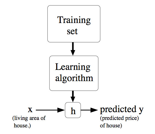
上表中面积和房间个数是输入参数，价格是所要输出的解。面积和房间个数分别表示一个特征，用X表示。价格用Y表示。表格的一行表示一个样本。现在要做的是根据这些样本来预测其他面积和房间个数对应的价格。可以用以下图来表示，即给定一个训练集合，学习函数h，使得h(x)能符合结果Y。

一. 批梯度下降算法 

可以用以下式子表示一个样本：

 

θ表示X映射成Y的权重，x表示一次特征。假设x₀=1,上式就可以写成：

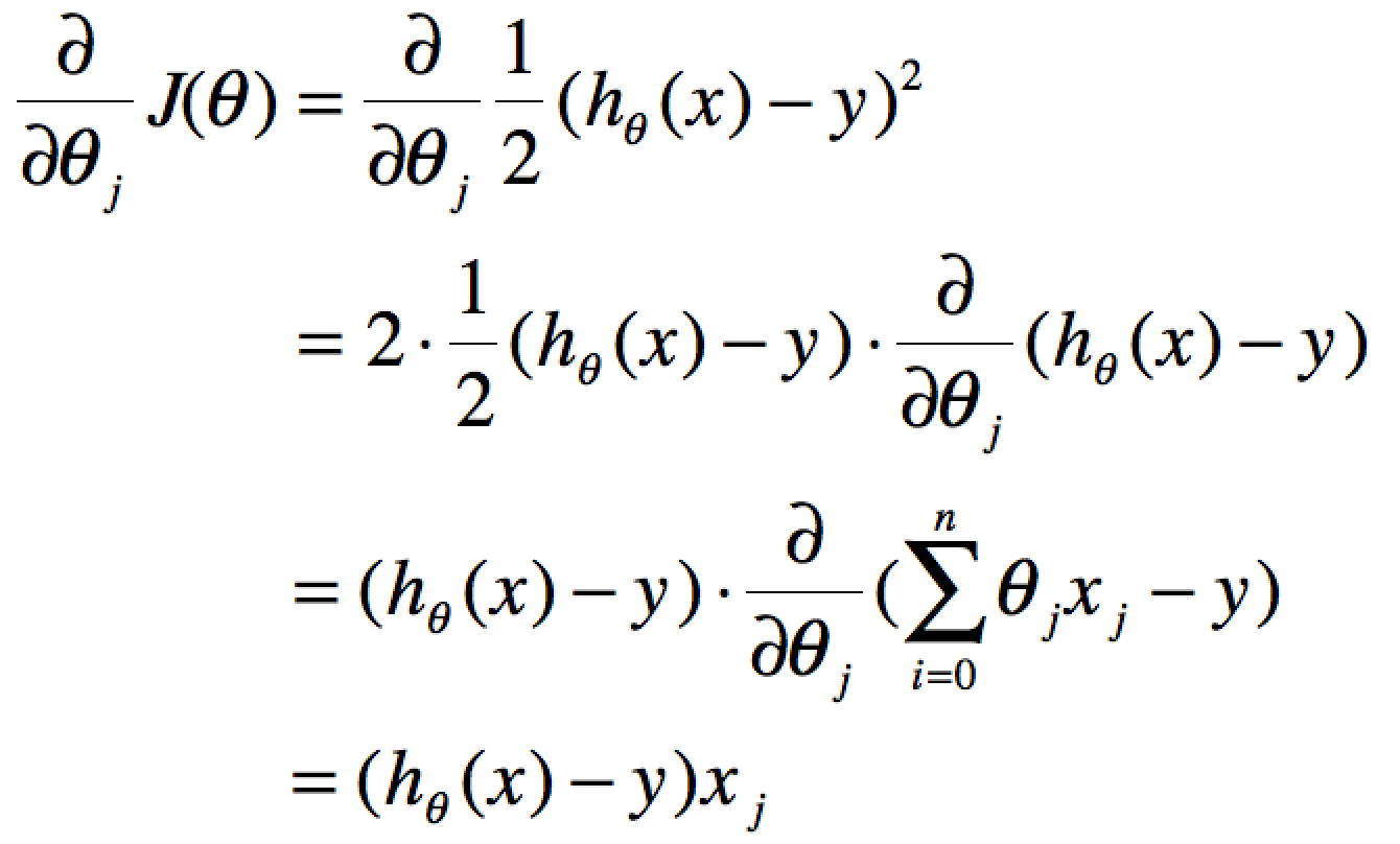
分别使用x^(j),y^(j)表示第J个样本。我们计算的目的是为了让计算的值无限接近真实值y，即代价函数可以采用LMS算法

要获取J(θ)最小，即对J(θ)进行求导且为零：

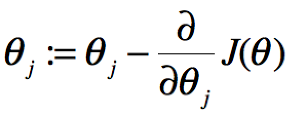
当单个特征值时，上式中j表示系数(权重)的编号，右边的值赋值给左边θ_j从而完成一次迭代。

单个特征的迭代如下：

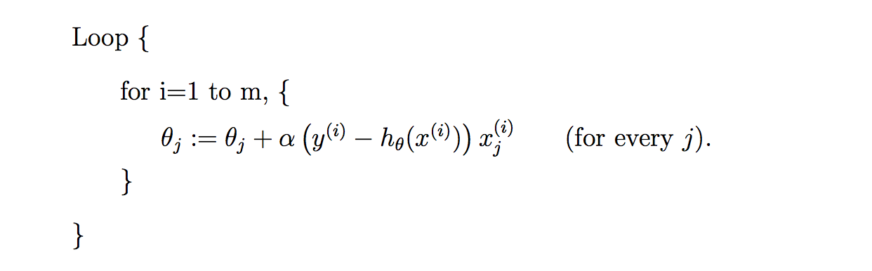
多个特征的迭代如下：

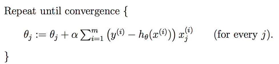
上式就是批梯度下降算法(batch gradient descent)，当上式收敛时则退出迭代，何为收敛，即前后两次迭代的值不再发生变化了。一般情况下，会设置一个具体的参数，当前后两次迭代差值小于该参数时候结束迭代。注意以下几点：

(1) a 即learning rate，决定的下降步伐，如果太小，则找到函数最小值的速度就很慢，如果太大，则可能会出现overshoot the minimum的现象；

 

(2) 初始点不同，获得的最小值也不同，因此梯度下降求得的只是局部最小值；

 

(3) 越接近最小值时，下降速度越慢；

 

(4) 计算批梯度下降算法时候，计算每一个θ值都需要遍历计算所有样本，当数据量的时候这是比较费时的计算。

 

批梯度下降算法的步骤可以归纳为以下几步：

 

(1)先确定向下一步的步伐大小，我们称为Learning rate ；

 

(2)任意给定一个初始值：θ向量，一般为0向量

 

(3)确定一个向下的方向，并向下走预先规定的步伐，并更新θ向量

 

(4)当下降的高度小于某个定义的值，则停止下降；

 

 

二. 随机梯度下降算法

因为每次计算梯度都需要遍历所有的样本点。这是因为梯度是J(θ)的导数，而J(θ)是需要考虑所有样本的误差和 ，这个方法问题就是，扩展性问题，当样本点很大的时候，基本就没法算了。所以接下来又提出了随机梯度下降算法(stochastic gradient descent )。随机梯度下降算法，每次迭代只是考虑让该样本点的J(θ)趋向最小，而不管其他的样本点，这样算法会很快，但是收敛的过程会比较曲折，整体效果上，大多数时候它只能接近局部最优解，而无法真正达到局部最优解。所以适合用于较大训练集的case。

三.代码实现

随机梯度下降算法的python的实现： 

 1 # coding=utf-8
 2 #!/usr/bin/python
 3 
 4 '''
 5 Created on 2014年9月6日
 6
 7 @author: Ryan C. F.
 8 
 9 '''
10 
11 #Training data set
12 #each element in x represents (x0,x1,x2)
13 x = [(1,0.,3) , (1,1.,3) ,(1,2.,3), (1,3.,2) , (1,4.,4)]
14 #y[i] is the output of y = theta0  x[0] + theta1  x[1] +theta2  x[2]
15 y = [95.364,97.217205,75.195834,60.105519,49.342380]
16 
17 
18 epsilon = 0.0001
19 #learning rate
20 alpha = 0.01
21 diff = [0,0]
22 error1 = 0
23 error0 =0
24 m = len(x)
25 
26 
27 #init the parameters to zero
28 theta0 = 0
29 theta1 = 0
30 theta2 = 0
31 
32 while True:
33 
34     #calculate the parameters
35     for i in range(m):
36
37         diff[0] = y[i]-( theta0 + theta1  x[i][1] + theta2  x[i][2] )
38
39         theta0 = theta0 + alpha  diff[0] x[i][0]
40         theta1 = theta1 + alpha  diff[0] x[i][1]
41         theta2 = theta2 + alpha  diff[0] x[i][2]
42
43     #calculate the cost function
44     error1 = 0
45     for lp in range(len(x)):
46         error1 += ( y[i]-( theta0 + theta1  x[i][1] + theta2  x[i][2] ) )*2/2
47
48     if abs(error1-error0) < epsilon:
49         break
50     else:
51         error0 = error1
52
53     print ' theta0 : %f, theta1 : %f, theta2 : %f, error1 : %f'%(theta0,theta1,theta2,error1)
54 
55 print 'Done: theta0 : %f, theta1 : %f, theta2 : %f'%(theta0,theta1,theta2)

批梯度下降算法

 1 # coding=utf-8
 2 #!/usr/bin/python
 3 
 4 '''
 5 Created on 2014年9月6日
 6
 7 @author: Ryan C. F.
 8 
 9 '''
10 
11 #Training data set
12 #each element in x represents (x0,x1,x2)
13 x = [(1,0.,3) , (1,1.,3) ,(1,2.,3), (1,3.,2) , (1,4.,4)]
14 #y[i] is the output of y = theta0  x[0] + theta1  x[1] +theta2  x[2]
15 y = [95.364,97.217205,75.195834,60.105519,49.342380]
16 
17 
18 epsilon = 0.000001
19 #learning rate
20 alpha = 0.001
21 diff = [0,0]
22 error1 = 0
23 error0 =0
24 m = len(x)
25 
26 #init the parameters to zero
27 theta0 = 0
28 theta1 = 0
29 theta2 = 0
30 sum0 = 0
31 sum1 = 0
32 sum2 = 0
33 while True:
34
35     #calculate the parameters
36     for i in range(m):
37         #begin batch gradient descent
38         diff[0] = y[i]-( theta0 + theta1  x[i][1] + theta2  x[i][2] )
39         sum0 = sum0 + alpha  diff[0] x[i][0]
40         sum1 = sum1 + alpha  diff[0] x[i][1]
41         sum2 = sum2 + alpha  diff[0] x[i][2]
42         #end  batch gradient descent
43     theta0 = sum0;
44     theta1 = sum1;
45     theta2 = sum2;
46     #calculate the cost function
47     error1 = 0
48     for lp in range(len(x)):
49         error1 += ( y[i]-( theta0 + theta1  x[i][1] + theta2  x[i][2] ) )*2/2
50
51     if abs(error1-error0) < epsilon:
52         break
53     else:
54         error0 = error1
55
56     print ' theta0 : %f, theta1 : %f, theta2 : %f, error1 : %f'%(theta0,theta1,theta2,error1)
57 
58 print 'Done: theta0 : %f, theta1 : %f, theta2 : %f'%(theta0,theta1,theta2)

通过上述批梯度下降和随机梯度下降算法代码的对比，不难发现两者的区别：

1. 随机梯度下降算法在迭代的时候，每迭代一个新的样本，就会更新一次所有的theta参数。

35     for i in range(m):
36
37         diff[0] = y[i]-( theta0 + theta1  x[i][1] + theta2  x[i][2] )
38
39         theta0 = theta0 + alpha  diff[0] x[i][0]
40         theta1 = theta1 + alpha  diff[0] x[i][1]
41         theta2 = theta2 + alpha  diff[0] x[i][2]

2. 批梯度下降算法在迭代的时候，是完成所有样本的迭代后才会去更新一次theta参数

35     #calculate the parameters
36     for i in range(m):
37         #begin batch gradient descent
38         diff[0] = y[i]-( theta0 + theta1  x[i][1] + theta2  x[i][2] )
39         sum0 = sum0 + alpha  diff[0] x[i][0]
40         sum1 = sum1 + alpha  diff[0] x[i][1]
41         sum2 = sum2 + alpha  diff[0] x[i][2]
42         #end  batch gradient descent
43     theta0 = sum0;
44     theta1 = sum1;
45     theta2 = sum2;

因此当样本数量很大时候，批梯度得做完所有样本的计算才能更新一次theta，从而花费的时间远大于随机梯度下降。但是随机梯度下降过早的结束了迭代，使得它获取的值只是接近局部最优解，而并非像批梯度下降算法那么是局部最优解。

因此我觉得以上的差别才是批梯度下降与随机梯度下降最本质的差别。