220430-三种短时傅立叶变换STFT的绘制及数据提取

• Figure

• Code

import numpy as np
import matplotlib.pyplot as plt
import scipy.signal as signal
# - [How to plot Spectrogram using STFT in python?](https://stackoverflow.com/questions/43109708/how-to-plot-spectrogram-using-stft-in-python/48205933#48205933)

sampling_rate = 8000.0
fft_size = 1024
step = fft_size/16
time = 2
t = np.arange(0, time, 1/sampling_rate)
sweep = signal.chirp(t, f0=100, t1=time, f1=0.8*sampling_rate/2, method='logarithmic')

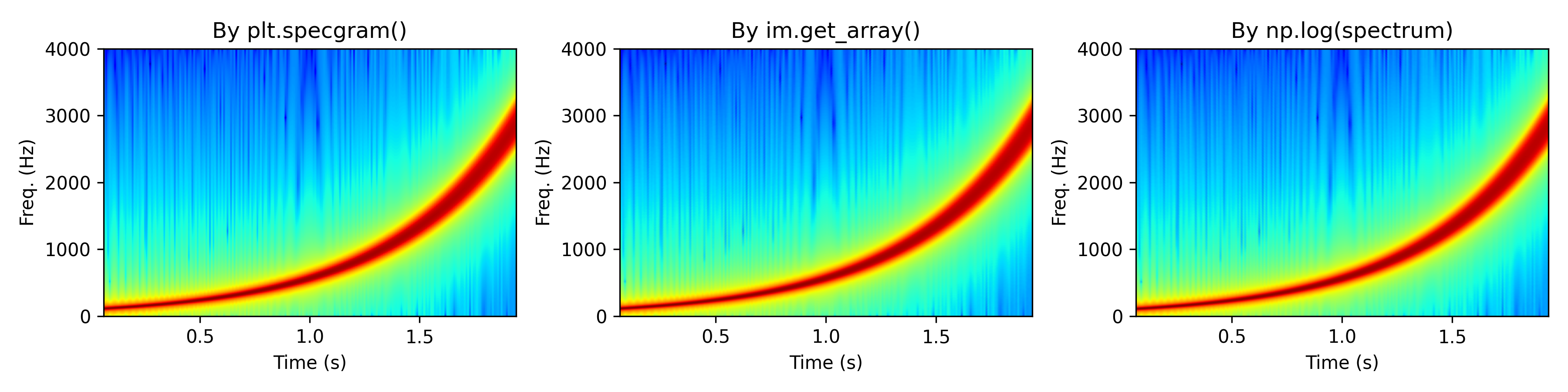
fig, ax = plt.subplots(1,3, figsize=(12, 3))
ax = ax.ravel()

# Figure 1
[spectrum, freqs, t, im] = ax[0].specgram(sweep, fft_size, sampling_rate, noverlap=1024-step, cmap='jet')
ax[0].set_xlabel('Time (s)')
ax[0].set_ylabel('Freq. (Hz)')
ax[0].set_title('By plt.specgram()')

# Figure 2
# plt.imshow(im.get_array(), cmap='jet', aspect='auto')
ax[1].pcolormesh(t, freqs[::-1], im.get_array(), cmap='jet', shading='gouraud')
ax[1].set_xlabel('Time (s)')
ax[1].set_ylabel('Freq. (Hz)')
ax[1].set_title('By im.get_array()')

# Figure 3
ax[2].pcolormesh(t, freqs, np.log(spectrum), cmap='jet', shading='gouraud')
ax[2].set_xlabel('Time (s)')
ax[2].set_ylabel('Freq. (Hz)')
ax[2].set_title('By np.log(spectrum)')

plt.tight_layout()
plt.savefig('output.png', dpi=300)

# Compare values
print(im.get_array()[:4, :4])
print('\n')
print(np.log(spectrum)[:4, :4])

• Comparison

[[-204.33209898 -219.84393176 -214.14525629 -203.59444001]
 [-201.31048748 -216.82498615 -210.87029865 -200.53882072]
 [-201.27672382 -216.79880707 -210.16099174 -200.40558268]
 [-201.22097657 -216.75575367 -209.18803361 -200.19223749]]
 
[[-22.84165273 -20.81034315 -21.35552053 -27.64431125]
 [-21.8274879  -20.04740739 -20.59310002 -24.67213702]
 [-21.15707948 -19.84181708 -20.38858459 -23.23503521]
 [-20.4209166  -19.50932131 -20.05665799 -22.21228083]]

• STFT vs. CWT

import numpy as np
import matplotlib.pyplot as plt
import scipy.signal as signal
# - [How to plot Spectrogram using STFT in python?](https://stackoverflow.com/questions/43109708/how-to-plot-spectrogram-using-stft-in-python/48205933#48205933)

fs = 1024
fft_size = 1024
step = fft_size/16
time=2
tt = np.arange(0, time, 1/fs) # 
# sweep = signal.chirp(t, f0=100, t1=time, f1=0.8*sampling_rate/2, method='logarithmic')
sweep = signal.chirp(tt, f0=30, t1=time, f1=500, method='quadratic')
print(len(sweep))

# fig, ax = plt.subplots(1,3,figsize=(24,6))
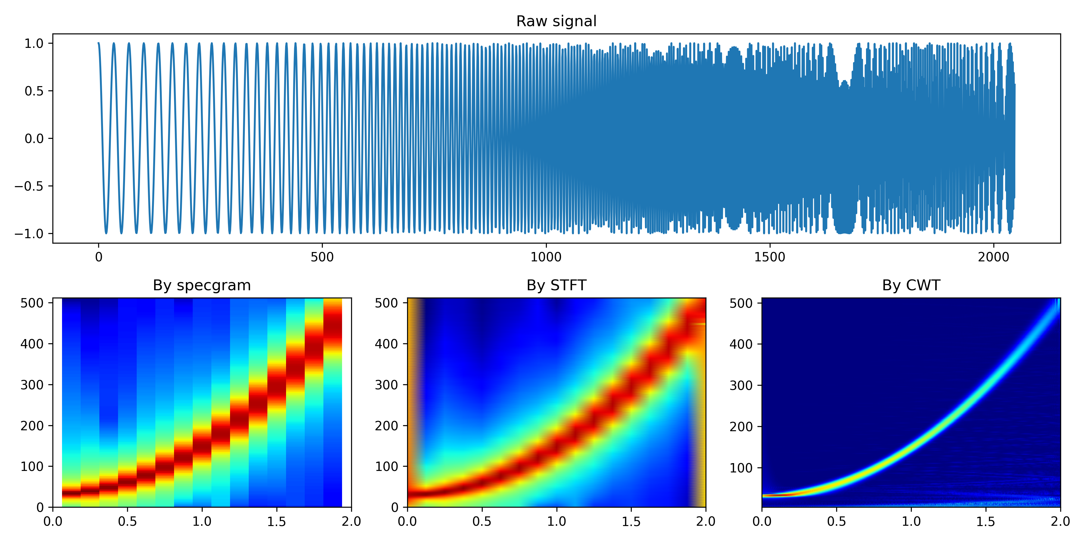
fig = plt.figure(figsize=(12,6))

# ax[0]
ax1 = plt.subplot(211)
ax1.plot(sweep)
ax1.set_title('Raw signal')

ax2 = plt.subplot(234)
[spectrum, freqs, t, im] = ax2.specgram(sweep, Fs=fs, cmap='jet')
ax2.set_xlim(0,2)
ax2.set_title('By specgram')

ax3 = plt.subplot(235)
f1, t1, Zxx = signal.stft(sweep, fs=fs)
ax3.pcolormesh(t1, f1, np.log(np.abs(Zxx)), shading='gouraud', cmap='jet') # vmin=0,  vmax=np.max(sweep),
ax3.set_title('By STFT')

ax4 = plt.subplot(236)
import pywt
wavename = 'cmor3-3'
totalscal = 256
fc = pywt.central_frequency(wavename)
cparam = 2 * fc * totalscal
scales = cparam / np.arange(totalscal, 1, -1)
[cwtmatr, frequencies] = pywt.cwt(sweep, scales, wavename, 1.0 / fs)
ax4.pcolormesh(tt, frequencies, np.abs(cwtmatr), shading='gouraud', cmap='jet') 
ax4.set_title('By CWT')
ax4.set_xlim(0,2)

plt.tight_layout()

• Reference
  How to plot Spectrogram using STFT in python?