


目录
1、使用pytorch的预定义算子来重新实现二分类任务。(必做)
2. 增加一个3个神经元的隐藏层,再次实现二分类,并与1做对比。(必做)
3. 自定义隐藏层层数和每个隐藏层中的神经元个数,尝试找到最优超参数完成二分 类。可以适当修改数据集,便于探索超参数。(选做)
自定义梯度计算和自动梯度计算:从计算性能、计算结果等多方面比较,谈谈自己的看法。
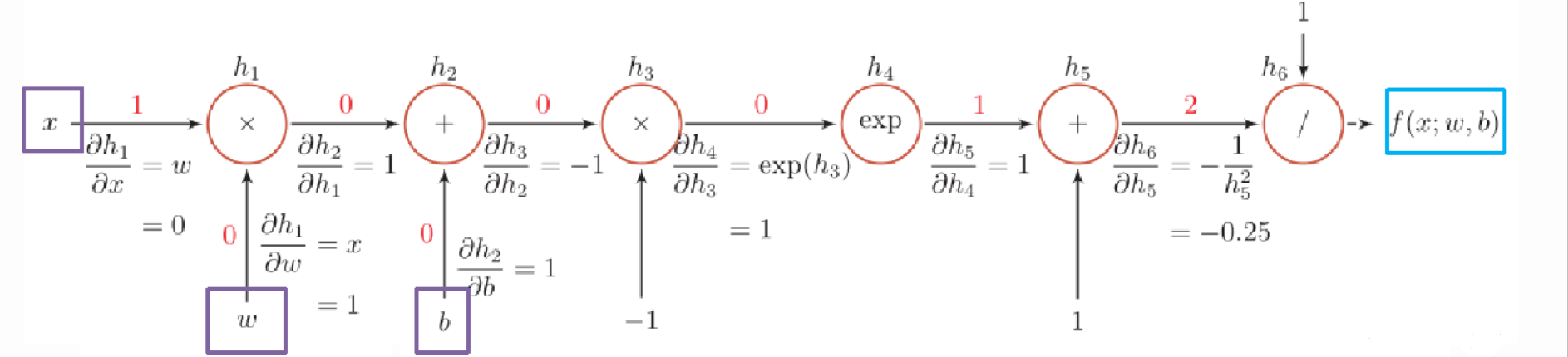
4.3 自动梯度计算
虽然我们能够通过模块化的方式比较好地对神经网络进行组装,但是每个模块的梯度计算过程仍然十分繁琐且容易出错。在深度学习框架中,已经封装了自动梯度计算的功能,我们只需要聚焦模型架构,不再需要耗费精力进行计算梯度。
飞桨提供了paddle.nn.Layer类,来方便快速的实现自己的层和模型。模型和层都可以基于paddle.nn.Layer扩充实现,模型只是一种特殊的层。继承了paddle.nn.Layer类的算子中,可以在内部直接调用其它继承paddle.nn.Layer类的算子,飞桨框架会自动识别算子中内嵌的paddle.nn.Layer类算子,并自动计算它们的梯度,并在优化时更新它们的参数。
pytorch中的相应内容是什么?请简要介绍。
4.3.1 利用预定义算子重新实现前馈神经网络
1、使用pytorch的预定义算子来重新实现二分类任务。(必做)
paddle.nn.Linear(in_features, out_features, weight_attr=None, bias_attr=None, name=None)
在paddle.nn.Linear里可以直接设置w和b,但是在torch.nn.Linear里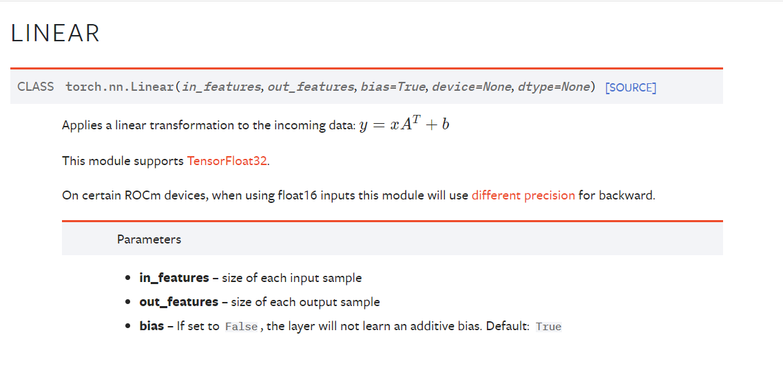
可以看到pytorch官网里给的Linear类中是不能设置w和b的,只能设置b的有没有,所以我在这里手动设置了一下w和b。
import torch.nn as nn
import torch.nn.functional as F
import os
import torch
from abc import abstractmethod
import math
import numpy as np
from make_moon import make_moons
from metric import accuracy
import matplotlib.pyplot as plt
from torch.nn.init  import normal_,constant_,uniform_
class Model_MLP_L2_V2(nn.Module):
    def __init__(self, input_size, hidden_size, output_size):
        super(Model_MLP_L2_V2, self).__init__()
        self.fc1 = nn.Linear(input_size, hidden_size)
        normal_(self.fc1.weight, mean=0., std=1.)
        constant_(self.fc1.bias, val=0.0)
        self.fc2 = nn.Linear(hidden_size, output_size)
        normal_(self.fc2.weight, mean=0., std=1.)
        constant_(self.fc2.bias, val=0.0)
        self.act_fn = torch.sigmoid

    # 前向计算
    def forward(self, inputs):
        z1 = self.fc1(inputs)
        a1 = self.act_fn(z1)
        z2 = self.fc2(a1)
        a2 = self.act_fn(z2)
        return a2
4.3.2 完善Runner类
class RunnerV2_2(object):
    def __init__(self, model, optimizer, metric, loss_fn, **kwargs):
        self.model = model
        self.optimizer = optimizer
        self.loss_fn = loss_fn
        self.metric = metric

        # 记录训练过程中的评估指标变化情况
        self.train_scores = []
        self.dev_scores = []

        # 记录训练过程中的评价指标变化情况
        self.train_loss = []
        self.dev_loss = []

    def train(self, train_set, dev_set, **kwargs):
        # 将模型切换为训练模式
        self.model.train()

        # 传入训练轮数,如果没有传入值则默认为0
        num_epochs = kwargs.get("num_epochs", 0)
        # 传入log打印频率,如果没有传入值则默认为100
        log_epochs = kwargs.get("log_epochs", 100)
        # 传入模型保存路径,如果没有传入值则默认为"best_model.pdparams"
        save_path = kwargs.get("save_path", "best_model.pdparams")

        # log打印函数,如果没有传入则默认为"None"
        custom_print_log = kwargs.get("custom_print_log", None)

        # 记录全局最优指标
        best_score = 0
        # 进行num_epochs轮训练
        for epoch in range(num_epochs):
            X, y = train_set
            # 获取模型预测
            logits = self.model(X)
            # 计算交叉熵损失
            trn_loss = self.loss_fn(logits, y)
            self.train_loss.append(trn_loss.item())
            # 计算评估指标
            trn_score = self.metric(logits, y).item()
            self.train_scores.append(trn_score)

            # 自动计算参数梯度
            trn_loss.backward()
            if custom_print_log is not None:
                # 打印每一层的梯度
                custom_print_log(self)

            # 参数更新
            self.optimizer.step()
            # 清空梯度
            self.optimizer.zero_grad()

            dev_score, dev_loss = self.evaluate(dev_set)
            # 如果当前指标为最优指标,保存该模型
            if dev_score > best_score:
                self.save_model(save_path)
                print(f"[Evaluate] best accuracy performence has been updated: {best_score:.5f} --> {dev_score:.5f}")
                best_score = dev_score

            if log_epochs and epoch % log_epochs == 0:
                print(f"[Train] epoch: {epoch}/{num_epochs}, loss: {trn_loss.item()}")

    # 模型评估阶段,使用'paddle.no_grad()'控制不计算和存储梯度
    @torch.no_grad()
    def evaluate(self, data_set):
        # 将模型切换为评估模式
        self.model.eval()

        X, y = data_set
        # 计算模型输出
        logits = self.model(X)
        # 计算损失函数
        loss = self.loss_fn(logits, y).item()
        self.dev_loss.append(loss)
        # 计算评估指标
        score = self.metric(logits, y).item()
        self.dev_scores.append(score)
        return score, loss

    def predict(self, X):
        # 将模型切换为评估模式
        self.model.eval()
        return self.model(X)

    # 使用'model.state_dict()'获取模型参数,并进行保存
    def save_model(self, saved_path):
        torch.save(self.model.state_dict(), saved_path)

    # 使用'model.set_state_dict'加载模型参数
    def load_model(self, model_path):
        state_dict = torch.load(model_path)
        self.model.load_state_dict(state_dict)
4.3.3 模型训练
# 设置模型
input_size = 2
hidden_size = 5
output_size = 1
model = Model_MLP_L2_V2(input_size=input_size, hidden_size=hidden_size, output_size=output_size)

# 设置损失函数
loss_fn = F.binary_cross_entropy

# 设置优化器
learning_rate = 0.2
optimizer = torch.optim.SGD(lr=learning_rate, params=model.parameters())

# 设置评价指标
metric = accuracy

# 其他参数
epoch_num = 1000
saved_path = 'best_model.pdparams'

# 实例化RunnerV2类,并传入训练配置
runner = RunnerV2_2(model, optimizer, metric, loss_fn)

runner.train([X_train, y_train], [X_dev, y_dev], num_epochs=epoch_num, log_epochs=50, save_path="best_model.pdparams")
得到以下结果:
[Evaluate] best accuracy performence has been updated: 0.00000 --> 0.45625
[Train] epoch: 0/1000, loss: 0.7848005294799805
[Evaluate] best accuracy performence has been updated: 0.45625 --> 0.47500
[Evaluate] best accuracy performence has been updated: 0.47500 --> 0.51875
[Evaluate] best accuracy performence has been updated: 0.51875 --> 0.56875
[Evaluate] best accuracy performence has been updated: 0.56875 --> 0.61875
[Evaluate] best accuracy performence has been updated: 0.61875 --> 0.65625
[Evaluate] best accuracy performence has been updated: 0.65625 --> 0.69375
[Evaluate] best accuracy performence has been updated: 0.69375 --> 0.71875
[Evaluate] best accuracy performence has been updated: 0.71875 --> 0.73750
[Evaluate] best accuracy performence has been updated: 0.73750 --> 0.74375
[Train] epoch: 50/1000, loss: 0.5194441080093384
[Evaluate] best accuracy performence has been updated: 0.74375 --> 0.75000
[Train] epoch: 100/1000, loss: 0.4518086016178131
[Evaluate] best accuracy performence has been updated: 0.75000 --> 0.75625
[Evaluate] best accuracy performence has been updated: 0.75625 --> 0.76250
[Evaluate] best accuracy performence has been updated: 0.76250 --> 0.76875
[Evaluate] best accuracy performence has been updated: 0.76875 --> 0.77500
[Evaluate] best accuracy performence has been updated: 0.77500 --> 0.78125
[Evaluate] best accuracy performence has been updated: 0.78125 --> 0.78750
[Evaluate] best accuracy performence has been updated: 0.78750 --> 0.80000
[Evaluate] best accuracy performence has been updated: 0.80000 --> 0.80625
[Train] epoch: 150/1000, loss: 0.40789881348609924
[Evaluate] best accuracy performence has been updated: 0.80625 --> 0.81250
[Evaluate] best accuracy performence has been updated: 0.81250 --> 0.81875
[Evaluate] best accuracy performence has been updated: 0.81875 --> 0.82500
[Evaluate] best accuracy performence has been updated: 0.82500 --> 0.83125
[Train] epoch: 200/1000, loss: 0.3763730525970459
[Train] epoch: 250/1000, loss: 0.353137344121933
[Evaluate] best accuracy performence has been updated: 0.83125 --> 0.83750
[Train] epoch: 300/1000, loss: 0.33587971329689026
[Evaluate] best accuracy performence has been updated: 0.83750 --> 0.84375
[Evaluate] best accuracy performence has been updated: 0.84375 --> 0.85000
[Train] epoch: 350/1000, loss: 0.32298415899276733
[Evaluate] best accuracy performence has been updated: 0.85000 --> 0.85625
[Train] epoch: 400/1000, loss: 0.31327566504478455
[Train] epoch: 450/1000, loss: 0.3059142827987671
[Train] epoch: 500/1000, loss: 0.3003050684928894
[Train] epoch: 550/1000, loss: 0.2960221767425537
[Train] epoch: 600/1000, loss: 0.29275229573249817
[Train] epoch: 650/1000, loss: 0.2902587354183197
[Train] epoch: 700/1000, loss: 0.2883586287498474
[Train] epoch: 750/1000, loss: 0.2869095206260681
[Train] epoch: 800/1000, loss: 0.28580060601234436
[Train] epoch: 850/1000, loss: 0.28494641184806824
[Train] epoch: 900/1000, loss: 0.2842817008495331
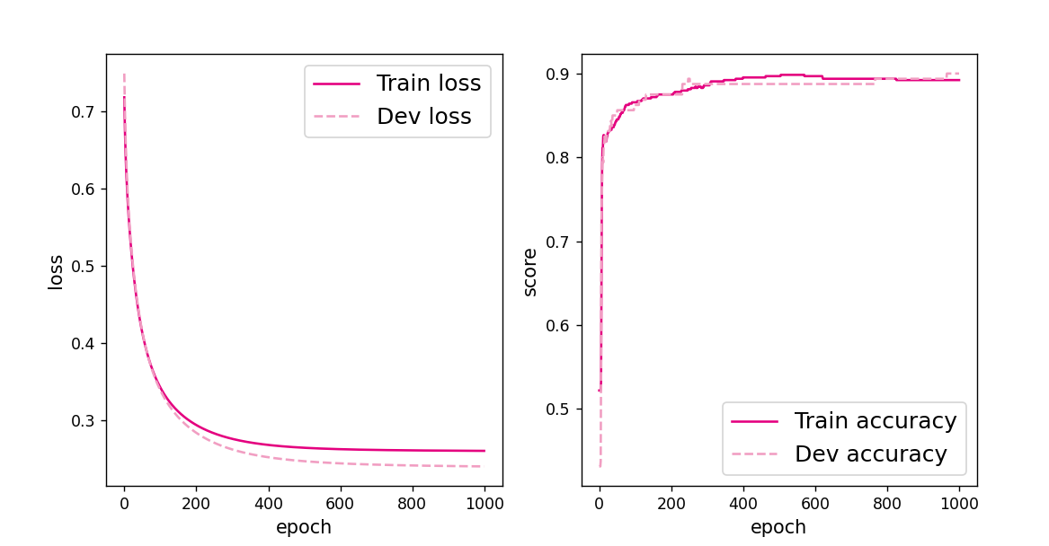
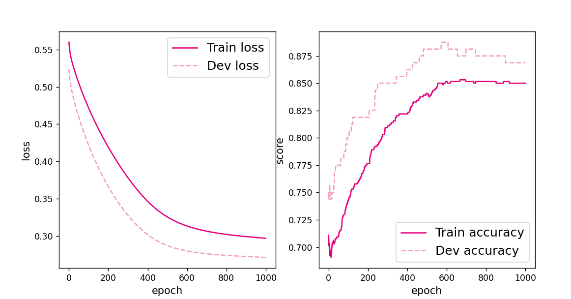
[Train] epoch: 950/1000, loss: 0.2837572693824768将训练过程中训练集与验证集的准确率变化情况进行可视化。
# 可视化观察训练集与验证集的指标变化情况
def plot(runner, fig_name):
    plt.figure(figsize=(10, 5))
    epochs = [i for i in range(len(runner.train_scores))]

    plt.subplot(1, 2, 1)
    plt.plot(epochs, runner.train_loss, color='#e4007f', label="Train loss")
    plt.plot(epochs, runner.dev_loss, color='#f19ec2', linestyle='--', label="Dev loss")
    # 绘制坐标轴和图例
    plt.ylabel("loss", fontsize='large')
    plt.xlabel("epoch", fontsize='large')
    plt.legend(loc='upper right', fontsize='x-large')

    plt.subplot(1, 2, 2)
    plt.plot(epochs, runner.train_scores, color='#e4007f', label="Train accuracy")
    plt.plot(epochs, runner.dev_scores, color='#f19ec2', linestyle='--', label="Dev accuracy")
    # 绘制坐标轴和图例
    plt.ylabel("score", fontsize='large')
    plt.xlabel("epoch", fontsize='large')
    plt.legend(loc='lower right', fontsize='x-large')

    plt.savefig(fig_name)
    plt.show()


plot(runner, 'fw-acc.pdf')
得到以下结果:
4.3.4 性能评价
# 模型评价
runner.load_model("best_model.pdparams")
score, loss = runner.evaluate([X_test, y_test])
print("[Test] score/loss: {:.4f}/{:.4f}".format(score, loss))
得到以下结果:
[Test] score/loss: 0.8400/0.35134.3.1 利用预定义算子重新实现前馈神经网络
2. 增加一个3个神经元的隐藏层,再次实现二分类,并与1做对比。(必做)
改变网络形状也需要改一下模型,如下:
class Model_MLP_L2_V2(nn.Module):
    def __init__(self, input_size, hidden_size,hidden_size2, output_size):
        super(Model_MLP_L2_V2, self).__init__()
        self.fc1 = nn.Linear(input_size, hidden_size)
        normal_(self.fc1.weight, mean=0., std=1.)
        constant_(self.fc1.bias, val=0.0)

        self.fc2 = nn.Linear(hidden_size, output_size)
        normal_(self.fc2.weight, mean=0., std=1.)
        constant_(self.fc2.bias, val=0.0)

        self.fc3 = nn.Linear(hidden_size2, output_size)
        normal_(self.fc3.weight, mean=0., std=1.)
        constant_(self.fc3.bias, val=0.0)

        self.act_fn = torch.sigmoid

    # 前向计算
    def forward(self, inputs):
        z1 = self.fc1(inputs.float())
        a1 = self.act_fn(z1)
        z2 = self.fc2(a1)
        a2 = self.act_fn(z2)
        return a2
# 设置模型
input_size = 2
hidden_size = 5
hidden_size2 = 3
output_size = 1
model = Model_MLP_L2_V4(input_size=input_size, hidden_size=hidden_size,hidden_size2=hidden_size2, output_size=output_size)
在我试了九九八十一次后得到训练结果大概就是这样的:
[Evaluate] best accuracy performence has been updated: 0.00000 --> 0.29375
[Train] epoch: 0/1000, loss: 0.754684567451477
[Evaluate] best accuracy performence has been updated: 0.29375 --> 0.31875
[Evaluate] best accuracy performence has been updated: 0.31875 --> 0.33750
[Evaluate] best accuracy performence has been updated: 0.33750 --> 0.35000
[Evaluate] best accuracy performence has been updated: 0.35000 --> 0.38750
[Evaluate] best accuracy performence has been updated: 0.38750 --> 0.43750
[Evaluate] best accuracy performence has been updated: 0.43750 --> 0.45000
[Evaluate] best accuracy performence has been updated: 0.45000 --> 0.50000
[Evaluate] best accuracy performence has been updated: 0.50000 --> 0.51250
[Evaluate] best accuracy performence has been updated: 0.51250 --> 0.52500
[Evaluate] best accuracy performence has been updated: 0.52500 --> 0.55000
[Evaluate] best accuracy performence has been updated: 0.55000 --> 0.56250
[Evaluate] best accuracy performence has been updated: 0.56250 --> 0.58750
[Evaluate] best accuracy performence has been updated: 0.58750 --> 0.61250
[Evaluate] best accuracy performence has been updated: 0.61250 --> 0.62500
[Evaluate] best accuracy performence has been updated: 0.62500 --> 0.65000
[Evaluate] best accuracy performence has been updated: 0.65000 --> 0.68125
[Evaluate] best accuracy performence has been updated: 0.68125 --> 0.69375
[Evaluate] best accuracy performence has been updated: 0.69375 --> 0.70625
[Evaluate] best accuracy performence has been updated: 0.70625 --> 0.71250
[Evaluate] best accuracy performence has been updated: 0.71250 --> 0.71875
[Evaluate] best accuracy performence has been updated: 0.71875 --> 0.73750
[Evaluate] best accuracy performence has been updated: 0.73750 --> 0.74375
[Evaluate] best accuracy performence has been updated: 0.74375 --> 0.75000
[Evaluate] best accuracy performence has been updated: 0.75000 --> 0.76250
[Evaluate] best accuracy performence has been updated: 0.76250 --> 0.76875
[Evaluate] best accuracy performence has been updated: 0.76875 --> 0.77500
[Evaluate] best accuracy performence has been updated: 0.77500 --> 0.78125
[Evaluate] best accuracy performence has been updated: 0.78125 --> 0.78750
[Evaluate] best accuracy performence has been updated: 0.78750 --> 0.79375
[Train] epoch: 50/1000, loss: 0.5374778509140015
[Evaluate] best accuracy performence has been updated: 0.79375 --> 0.80000
[Train] epoch: 100/1000, loss: 0.4248269498348236
[Evaluate] best accuracy performence has been updated: 0.80000 --> 0.80625
[Evaluate] best accuracy performence has been updated: 0.80625 --> 0.81250
[Evaluate] best accuracy performence has been updated: 0.81250 --> 0.81875
[Evaluate] best accuracy performence has been updated: 0.81875 --> 0.82500
[Evaluate] best accuracy performence has been updated: 0.82500 --> 0.83125
[Train] epoch: 150/1000, loss: 0.36857840418815613
[Evaluate] best accuracy performence has been updated: 0.83125 --> 0.83750
[Evaluate] best accuracy performence has been updated: 0.83750 --> 0.84375
[Train] epoch: 200/1000, loss: 0.33738794922828674
[Evaluate] best accuracy performence has been updated: 0.84375 --> 0.85000
[Evaluate] best accuracy performence has been updated: 0.85000 --> 0.85625
[Train] epoch: 250/1000, loss: 0.3170816898345947
[Train] epoch: 300/1000, loss: 0.30261653661727905
[Evaluate] best accuracy performence has been updated: 0.85625 --> 0.86250
[Evaluate] best accuracy performence has been updated: 0.86250 --> 0.86875
[Train] epoch: 350/1000, loss: 0.292058527469635
[Train] epoch: 400/1000, loss: 0.28439122438430786
[Train] epoch: 450/1000, loss: 0.2788788080215454
[Train] epoch: 500/1000, loss: 0.27493661642074585
[Train] epoch: 550/1000, loss: 0.2721155285835266
[Train] epoch: 600/1000, loss: 0.27008694410324097
[Train] epoch: 650/1000, loss: 0.26861780881881714
[Train] epoch: 700/1000, loss: 0.26754504442214966
[Train] epoch: 750/1000, loss: 0.26675477623939514
[Train] epoch: 800/1000, loss: 0.26616689562797546
[Train] epoch: 850/1000, loss: 0.26572513580322266
[Train] epoch: 900/1000, loss: 0.26538926362991333
[Evaluate] best accuracy performence has been updated: 0.86875 --> 0.87500
[Train] epoch: 950/1000, loss: 0.26513057947158813
[Test] score/loss: 0.8550/0.2731

进程已结束,退出代码为 0
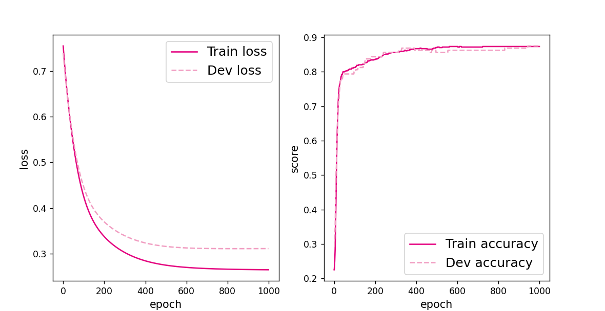
添加了一个三个神经元的隐藏层后发现训练结果和1相比差不多,虽然偶尔会有一个比较高,但是大部分就是我展示出来的结果这样比1的效果要好一点,但是也没有高很多。我又改了一下学习率把学习率改成1,lr=1
得到以下结果:
[Evaluate] best accuracy performence has been updated: 0.93750 --> 0.94375
[Evaluate] best accuracy performence has been updated: 0.94375 --> 0.95000
[Train] epoch: 950/1000, loss: 0.15602488815784454
[Test] score/loss: 0.9400/0.1560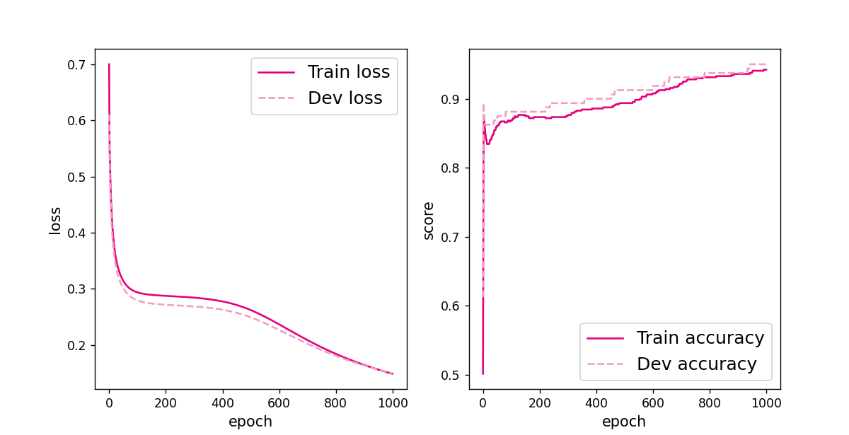
发现这个效果一下就上去了,但是我又多测试了几次发现并不稳定,就比如这一次:
[Evaluate] best accuracy performence has been updated: 0.86250 --> 0.86875
[Train] epoch: 150/1000, loss: 0.2642468810081482
[Train] epoch: 200/1000, loss: 0.2615928053855896
[Train] epoch: 250/1000, loss: 0.26074686646461487
[Train] epoch: 300/1000, loss: 0.26030269265174866
[Train] epoch: 350/1000, loss: 0.25997406244277954
[Train] epoch: 400/1000, loss: 0.2596961557865143
[Train] epoch: 450/1000, loss: 0.2594510018825531
[Train] epoch: 500/1000, loss: 0.25923141837120056
[Train] epoch: 550/1000, loss: 0.2590330243110657
[Train] epoch: 600/1000, loss: 0.25885269045829773
[Train] epoch: 650/1000, loss: 0.2586878538131714
[Train] epoch: 700/1000, loss: 0.2585364878177643
[Train] epoch: 750/1000, loss: 0.25839686393737793
[Train] epoch: 800/1000, loss: 0.2582675814628601
[Train] epoch: 850/1000, loss: 0.25814738869667053
[Train] epoch: 900/1000, loss: 0.2580353021621704
[Train] epoch: 950/1000, loss: 0.25793033838272095
[Test] score/loss: 0.8550/0.3199

进程已结束,退出代码为 0
效果并没有提升甚至还下降了,不过学习率上升了以后大部分时间效果还是比较好的,这种情况是比较特殊的。我又把学习率往上调了一下,lr=3,得到以下结果:
[Evaluate] best accuracy performence has been updated: 0.99375 --> 1.00000
[Train] epoch: 900/1000, loss: 0.040740884840488434
[Train] epoch: 950/1000, loss: 0.03657595440745354
[Test] score/loss: 0.9950/0.0440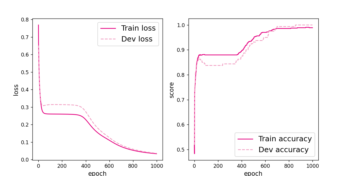
果然学习率上去了,结果也稳定了,效果也好了。
3. 自定义隐藏层层数和每个隐藏层中的神经元个数,尝试找到最优超参数完成二分 类。可以适当修改数据集,便于探索超参数。(选做)
虽然说是自定义层数和神经元个数,但是也要有个方向,要知道怎么去定义。
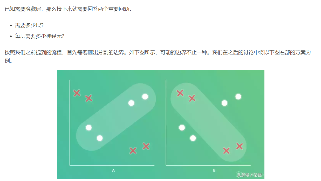
 再往下的我就不复制了,这里参考博客:https://www.toutiao.com/a6615751007013962244/
这里有几个公式:
- 隐藏神经元的数量应在输入层的大小和输出层的大小之间。
- 隐藏神经元的数量应为输入层大小的2/3加上输出层大小的2/3。
- 隐藏神经元的数量应小于输入层大小的两倍。
因为这是一个二分类问题,所以我认为隐藏层有一个或者两个就可以了,然后我们进行神经元的设置。
先是一个隐藏层5个神经元,也就是上面写过的结果:
[Test] score/loss: 0.8250/0.3510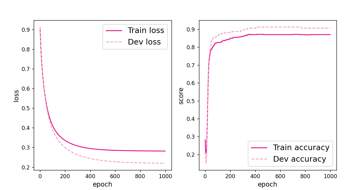
变成4个神经元:
[Test] score/loss: 0.9000/0.2668
3个神经元:
[Test] score/loss: 0.8350/0.5627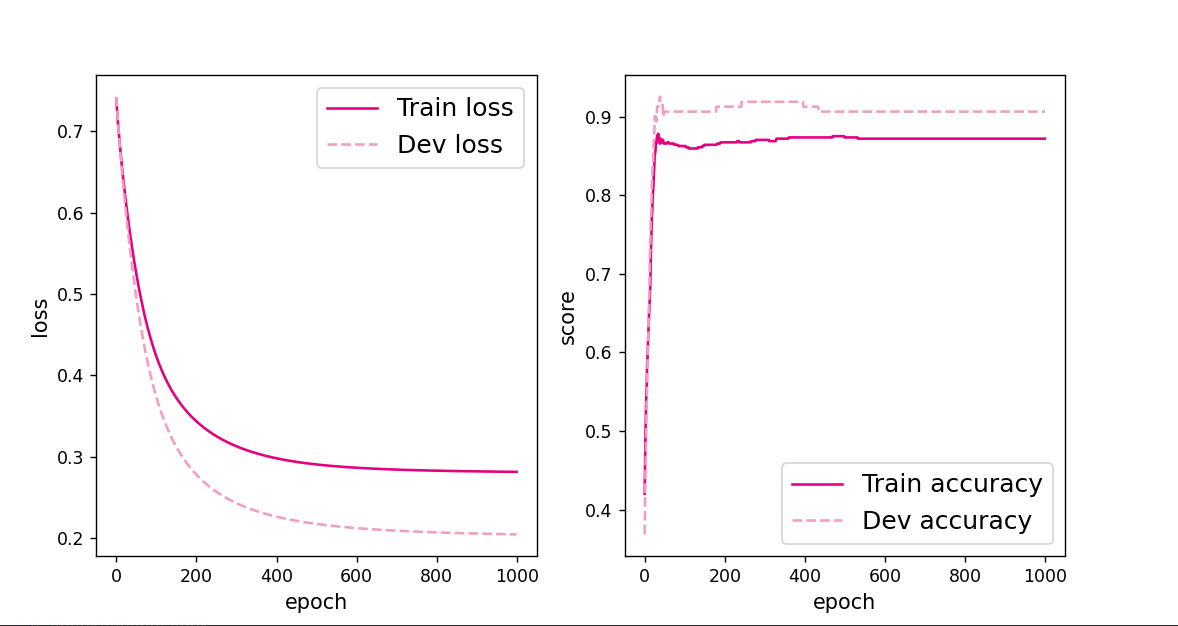
2个神经元: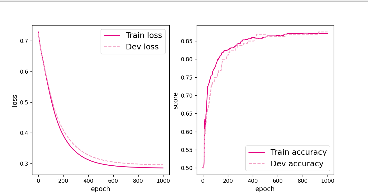
[Test] score/loss: 0.9100/0.2403我们再换到2个隐藏层神经元分别是5和3也就是上面写过的:
[Test] score/loss: 0.8550/0.3455
从上述的发现隐藏层1个神经元2个的时候效果是最好的,但是对比于上面更改学习率来说,这点提升好像有点少,所以我把一个隐藏层两个神经元的情况下学习率更改为2:
[Test] score/loss: 0.8550/0.3369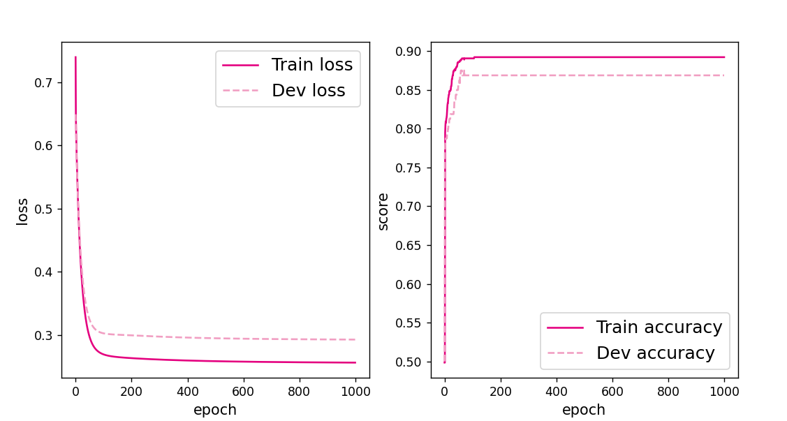
效果反而下降了,这是为什么??
我又把学习率改成3:
[Test] score/loss: 0.8750/0.2995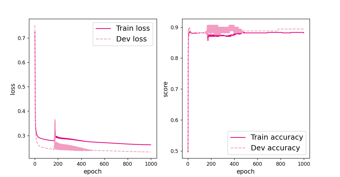
发现还是没有很大的变化,然后我又把神经元个数变回5个,然后学习率lr=2:
[Test] score/loss: 0.9850/0.0816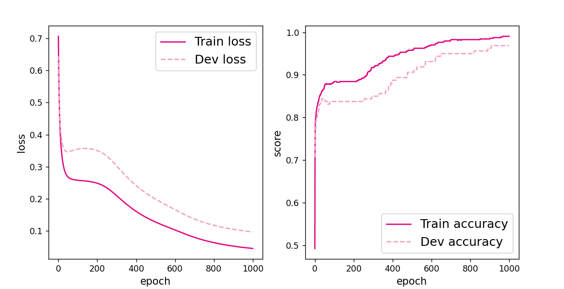
发现不如上面的lr=3,但是上面lr=3时效果并不稳定,所以我改成lr=5: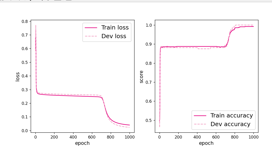
[Evaluate] best accuracy performence has been updated: 0.99375 --> 1.00000
[Train] epoch: 850/1000, loss: 0.07662317156791687
[Train] epoch: 900/1000, loss: 0.06233246996998787
[Train] epoch: 950/1000, loss: 0.05472086742520332
[Test] score/loss: 1.0000/0.0596
emmmm ,这应该就可以确定隐藏层是1个神经元是5个学习率lr=5的时候效果最好了
【思考题】
自定义梯度计算和自动梯度计算:从计算性能、计算结果等多方面比较,谈谈自己的看法。
在PyTorch中,torch.Tensor类是存储和变换数据的重要工具,相比于Numpy,Tensor提供GPU计算和自动求梯度等更多功能,在深度学习中,我们经常需要对函数求梯度(gradient)。PyTorch提供的autograd包能够根据输入和前向传播过程自动构建计算图,并执行反向传播。
Tensor是这个pytorch的自动求导部分的核心类,如果将其属性.requires_grad=True,它将开始追踪(track) 在该tensor上的所有操作,从而实现利用链式法则进行的梯度传播。完成计算后,可以调用.backward()来完成所有梯度计算。此Tensor的梯度将累积到.grad属性中。
如果不想要被继续对tensor进行追踪,可以调用.detach()将其从追踪记录中分离出来,接下来的梯度就传不过去了。此外,还可以用with torch.no_grad()将不想被追踪的操作代码块包裹起来,这种方法在评估模型的时候很常用,因为此时并不需要继续对梯度进行计算。
Function是另外一个很重要的类。Tensor和Function互相结合就可以构建一个记录有整个计算过程的有向无环图(DAG)。每个Tensor都有一个.grad_fn属性,该属性即创建该Tensor的Function, 就是说该Tensor是不是通过某些运算得到的,若是,则grad_fn返回一个与这些运算相关的对象,否则是None。
我们上次实验是用的自定义梯度计算,这次实验用的是自动梯度计算。所以我们可以将这两次的性能和结果来进行对比。
自定义梯度计算:
    def backward(self):
        # 计算损失函数对模型预测的导数
        loss_grad_predicts = -1.0 * (self.labels / self.predicts -
                                     (1 - self.labels) / (1 - self.predicts)) / self.num

        # 梯度反向传播
        self.model.backward(loss_grad_predicts)
得到的结果:
[Test] score/loss: 0.7750/0.4362而自动梯度计算:
     # 自动计算参数梯度
            trn_loss.backward()
得到的结果:
[Test] score/loss: 0.9000/0.2246
发现自动梯度计算的效果要好一点,然后我们再测试一下两者所用时间:
自定义梯度计算:
运行时间: 0.9484963417053223自动梯度计算:
运行时间: 0.7904136180877686发现自动梯度计算不管从时间还是结果上都要优于自定义梯度计算,
4.4 优化问题
4.4.1 参数初始化
实现一个神经网络前,需要先初始化模型参数。
如果对每一层的权重和偏置都用0初始化,那么通过第一遍前向计算,所有隐藏层神经元的激活值都相同;在反向传播时,所有权重的更新也都相同,这样会导致隐藏层神经元没有差异性,出现对称权重现象。
class Model_MLP_L2_V4(nn.Module):
    def __init__(self, input_size, hidden_size, output_size):
        super(Model_MLP_L2_V4, self).__init__()
        # 使用'paddle.nn.Linear'定义线性层。
        # 其中in_features为线性层输入维度;out_features为线性层输出维度
        # weight_attr为权重参数属性
        # bias_attr为偏置参数属性

        self.fc1 = nn.Linear(input_size, hidden_size)
        constant_(self.fc1.weight, val=0.0)
        constant_(self.fc1.bias, val=0.0)
        self.fc2 = nn.Linear(hidden_size, output_size)
        constant_(self.fc2.weight, val=0.0)
        constant_(self.fc2.bias, val=0.0)
        self.act_fn = torch.sigmoid

        # 使用'paddle.nn.functional.sigmoid'定义 Logistic 激活函数
        self.act_fn = torch.sigmoid

    # 前向计算
    def forward(self, inputs):
        z1 = self.fc1(inputs.float())
        a1 = self.act_fn(z1)
        z2 = self.fc2(a1)
        a2 = self.act_fn(z2)
        return a2


def print_weights(runner):
    print('The weights of the Layers:')
    for item in runner.model.named_parameters():
        print(item)
利用Runner类训练模型:
# 设置模型
input_size = 2
hidden_size = 5
output_size = 1
model = Model_MLP_L2_V4(input_size=input_size, hidden_size=hidden_size, output_size=output_size)

# 设置损失函数
loss_fn = F.binary_cross_entropy

# 设置优化器
learning_rate = 0.2 #5e-2
optimizer = torch.optim.SGD(lr=learning_rate, params=model.parameters())

# 设置评价指标
metric = accuracy

# 其他参数
epoch = 2000
saved_path = 'best_model.pdparams'

# 实例化RunnerV2类,并传入训练配置
runner = RunnerV2_2(model, optimizer, metric, loss_fn)

runner.train([X_train, y_train], [X_dev, y_dev], num_epochs=5, log_epochs=50, save_path="best_model.pdparams",custom_print_log=print_weights)
可视化训练和验证集上的主准确率和loss变化:
plot(runner, "fw-zero.pdf")得到以下结果:
The weights of the Layers:
('fc1.weight', Parameter containing:
tensor([[0., 0.],
        [0., 0.],
        [0., 0.],
        [0., 0.],
        [0., 0.]], requires_grad=True))
('fc1.bias', Parameter containing:
tensor([0., 0., 0., 0., 0.], requires_grad=True))
('fc2.weight', Parameter containing:
tensor([[0., 0., 0., 0., 0.]], requires_grad=True))
('fc2.bias', Parameter containing:
tensor([0.], requires_grad=True))
[Evaluate] best accuracy performence has been updated: 0.00000 --> 0.48750
[Train] epoch: 0/5, loss: 0.6931473016738892
The weights of the Layers:
('fc1.weight', Parameter containing:
tensor([[0., 0.],
        [0., 0.],
        [0., 0.],
        [0., 0.],
        [0., 0.]], requires_grad=True))
('fc1.bias', Parameter containing:
tensor([0., 0., 0., 0., 0.], requires_grad=True))
('fc2.weight', Parameter containing:
tensor([[-0.0020, -0.0020, -0.0020, -0.0020, -0.0020]], requires_grad=True))
('fc2.bias', Parameter containing:
tensor([-0.0041], requires_grad=True))
The weights of the Layers:
('fc1.weight', Parameter containing:
tensor([[-2.2723e-05,  1.9955e-05],
        [-2.2723e-05,  1.9955e-05],
        [-2.2723e-05,  1.9955e-05],
        [-2.2723e-05,  1.9955e-05],
        [-2.2723e-05,  1.9955e-05]], requires_grad=True))
('fc1.bias', Parameter containing:
tensor([1.8309e-06, 1.8309e-06, 1.8309e-06, 1.8309e-06, 1.8309e-06],
       requires_grad=True))
('fc2.weight', Parameter containing:
tensor([[-0.0038, -0.0038, -0.0038, -0.0038, -0.0038]], requires_grad=True))
('fc2.bias', Parameter containing:
tensor([-0.0077], requires_grad=True))
The weights of the Layers:
('fc1.weight', Parameter containing:
tensor([[-6.5808e-05,  5.7519e-05],
        [-6.5808e-05,  5.7519e-05],
        [-6.5808e-05,  5.7519e-05],
        [-6.5808e-05,  5.7519e-05],
        [-6.5808e-05,  5.7519e-05]], requires_grad=True))
('fc1.bias', Parameter containing:
tensor([4.8980e-06, 4.8980e-06, 4.8980e-06, 4.8980e-06, 4.8980e-06],
       requires_grad=True))
('fc2.weight', Parameter containing:
tensor([[-0.0054, -0.0054, -0.0054, -0.0054, -0.0054]], requires_grad=True))
('fc2.bias', Parameter containing:
tensor([-0.0109], requires_grad=True))
The weights of the Layers:
('fc1.weight', Parameter containing:
tensor([[-0.0001,  0.0001],
        [-0.0001,  0.0001],
        [-0.0001,  0.0001],
        [-0.0001,  0.0001],
        [-0.0001,  0.0001]], requires_grad=True))
('fc1.bias', Parameter containing:
tensor([8.7562e-06, 8.7562e-06, 8.7562e-06, 8.7562e-06, 8.7562e-06],
       requires_grad=True))
('fc2.weight', Parameter containing:
tensor([[-0.0069, -0.0069, -0.0069, -0.0069, -0.0069]], requires_grad=True))
('fc2.bias', Parameter containing:
tensor([-0.0137], requires_grad=True))

进程已结束,退出代码为 0

从输出结果看,二分类准确率为50%左右,说明模型没有学到任何内容。训练和验证loss几乎没有怎么下降。
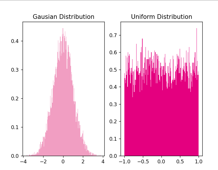
为了避免对称权重现象,可以使用高斯分布或均匀分布初始化神经网络的参数。
高斯分布和均匀分布采样的实现和可视化代码如下:
# 使用'paddle.normal'实现高斯分布采样,其中'mean'为高斯分布的均值,'std'为高斯分布的标准差,'shape'为输出形状
gausian_weights = torch.normal(mean=0.0, std=1.0, size=[10000])
# 使用'paddle.uniform'实现在[min,max)范围内的均匀分布采样,其中'shape'为输出形状
uniform_weights = torch.Tensor(10000)
uniform_weights.uniform_(-1,1)
print(uniform_weights)
# 绘制两种参数分布
plt.figure()
plt.subplot(1,2,1)
plt.title('Gausian Distribution')
plt.hist(gausian_weights, bins=200, density=True, color='#f19ec2')
plt.subplot(1,2,2)
plt.title('Uniform Distribution')
plt.hist(uniform_weights, bins=200, density=True, color='#e4007f')
plt.savefig('fw-gausian-uniform.pdf')
plt.show()
4.4.2 梯度消失问题
在神经网络的构建过程中,随着网络层数的增加,理论上网络的拟合能力也应该是越来越好的。但是随着网络变深,参数学习更加困难,容易出现梯度消失问题。
由于Sigmoid型函数的饱和性,饱和区的导数更接近于0,误差经过每一层传递都会不断衰减。当网络层数很深时,梯度就会不停衰减,甚至消失,使得整个网络很难训练,这就是所谓的梯度消失问题。
在深度神经网络中,减轻梯度消失问题的方法有很多种,一种简单有效的方式就是使用导数比较大的激活函数,如:ReLU。
4.4.2.1 模型构建
定义一个前馈神经网络,包含4个隐藏层和1个输出层,通过传入的参数指定激活函数。代码实现如下:
# 定义多层前馈神经网络
class Model_MLP_L5(nn.Module):
    def __init__(self, input_size, output_size, act='sigmoid', w_init=torch.normal(mean=torch.tensor(0.0), std=torch.tensor(0.01)), b_init=torch.tensor(1.0)):
        super(Model_MLP_L5, self).__init__()
        self.fc1 = torch.nn.Linear(input_size, 3)
        self.fc2 = torch.nn.Linear(3, 3)
        self.fc3 = torch.nn.Linear(3, 3)
        self.fc4 = torch.nn.Linear(3, 3)
        self.fc5 = torch.nn.Linear(3, output_size)
        # 定义网络使用的激活函数
        if act == 'sigmoid':
            self.act = F.sigmoid
        elif act == 'relu':
            self.act = F.relu
        elif act == 'lrelu':
            self.act = F.leaky_relu
        else:
            raise ValueError("Please enter sigmoid relu or lrelu!")
        # 初始化线性层权重和偏置参数
        self.init_weights(w_init, b_init)

    # 初始化线性层权重和偏置参数
    def init_weights(self, w_init, b_init):
        # 使用'named_sublayers'遍历所有网络层
        for n, m in self.named_parameters():
            # 如果是线性层,则使用指定方式进行参数初始化
            if isinstance(m, nn.Linear):
                w_init(m.weight)
                b_init(m.bias)

    def forward(self, inputs):
        outputs = self.fc1(inputs)
        outputs = self.act(outputs)
        outputs = self.fc2(outputs)
        outputs = self.act(outputs)
        outputs = self.fc3(outputs)
        outputs = self.act(outputs)
        outputs = self.fc4(outputs)
        outputs = self.act(outputs)
        outputs = self.fc5(outputs)
        outputs = F.sigmoid(outputs)
        return outputs
4.4.2.2 使用Sigmoid型函数进行训练
使用Sigmoid型函数作为激活函数,为了便于观察梯度消失现象,只进行一轮网络优化。代码实现如下:
定义梯度打印函数
def print_grads(runner):
    # 打印每一层的权重的模
    print('The gradient of the Layers:')
    for name,item in runner.model.named_parameters():
        if(len(item.size())==2):
             print(item)
             print(name,torch.norm(input=item,p=2))
             # 学习率大小
lr = 0.01
# 定义网络,激活函数使用sigmoid
model =  Model_MLP_L5(input_size=2, output_size=1, act='sigmoid')
# 定义优化器
optimizer = torch.optim.SGD(lr=lr, params=model.parameters())
# 定义损失函数,使用交叉熵损失函数
loss_fn = F.binary_cross_entropy
# 定义评价指标
metric = accuracy
# 指定梯度打印函数
custom_print_log=print_grads
实例化RunnerV2_2类,并传入训练配置。代码实现如下:
# 实例化Runner类
runner = RunnerV2_2(model, optimizer, metric, loss_fn)
模型训练,打印网络每层梯度值的ℓ2ℓ2范数。代码实现如下:
# 启动训练
runner.train([X_train, y_train], [X_dev, y_dev],
            num_epochs=1, log_epochs=None,
            save_path="best_model.pdparams",
            custom_print_log=custom_print_log)
得到以下结果:
The gradient of the Layers:
Parameter containing:
tensor([[ 0.2164,  0.1399],
        [ 0.6758, -0.0936],
        [ 0.5075, -0.6908]], requires_grad=True)
fc1.weight tensor(1.1255, grad_fn=<NormBackward1>)
Parameter containing:
tensor([[-0.5121, -0.2570, -0.4033],
        [ 0.4516,  0.3644, -0.1825],
        [ 0.3609, -0.1477,  0.2830]], requires_grad=True)
fc2.weight tensor(1.0455, grad_fn=<NormBackward1>)
Parameter containing:
tensor([[ 0.2767,  0.4889,  0.1055],
        [-0.4200,  0.1725, -0.5390],
        [-0.4808,  0.2739, -0.4394]], requires_grad=True)
fc3.weight tensor(1.1501, grad_fn=<NormBackward1>)
Parameter containing:
tensor([[ 0.5159,  0.3937, -0.2794],
        [-0.4812,  0.2626, -0.5522],
        [ 0.4008, -0.2584,  0.1896]], requires_grad=True)
fc4.weight tensor(1.1696, grad_fn=<NormBackward1>)
Parameter containing:
tensor([[-0.4302, -0.4532, -0.0690]], requires_grad=True)
fc5.weight tensor(0.6286, grad_fn=<NormBackward1>)
[Evaluate] best accuracy performence has been updated: 0.00000 --> 0.36875

进程已结束,退出代码为 0
观察实验结果可以发现,梯度经过每一个神经层的传递都会不断衰减,最终传递到第一个神经层时,梯度几乎完全消失。
4.4.2.3 使用ReLU函数进行模型训练
lr = 0.01  # 学习率大小

# 定义网络,激活函数使用relu
model =  Model_MLP_L5(input_size=2, output_size=1, act='relu')

# 定义优化器
optimizer = torch.optim.SGD(lr=lr, params=model.parameters())

# 定义损失函数
# 定义损失函数,这里使用交叉熵损失函数
loss_fn = F.binary_cross_entropy

# 定义评估指标
metric = accuracy

# 实例化Runner
runner = RunnerV2_2(model, optimizer, metric, loss_fn)

# 启动训练
runner.train([X_train, y_train], [X_dev, y_dev],
            num_epochs=1, log_epochs=None,
            save_path="best_model.pdparams",
            custom_print_log=custom_print_log)
得到以下结果:
The gradient of the Layers:
Parameter containing:
tensor([[-0.0650,  0.3647],
        [ 0.1154, -0.6875],
        [-0.6200,  0.3741]], requires_grad=True)
fc1.weight tensor(1.0712, grad_fn=<NormBackward1>)
Parameter containing:
tensor([[ 0.4844,  0.2058, -0.0677],
        [-0.1264,  0.5368,  0.1555],
        [-0.5234, -0.3148, -0.2681]], requires_grad=True)
fc2.weight tensor(1.0270, grad_fn=<NormBackward1>)
Parameter containing:
tensor([[ 0.0585,  0.1545,  0.3562],
        [ 0.0751,  0.1382, -0.3609],
        [ 0.4400, -0.4026,  0.2186]], requires_grad=True)
fc3.weight tensor(0.8442, grad_fn=<NormBackward1>)
Parameter containing:
tensor([[-0.3096, -0.4293,  0.2616],
        [ 0.5773,  0.3067,  0.1469],
        [ 0.2019,  0.4589,  0.5674]], requires_grad=True)
fc4.weight tensor(1.1708, grad_fn=<NormBackward1>)
Parameter containing:
tensor([[-0.3251, -0.2534,  0.4465]], requires_grad=True)
fc5.weight tensor(0.6077, grad_fn=<NormBackward1>)
[Evaluate] best accuracy performence has been updated: 0.00000 --> 0.51250

进程已结束,退出代码为 0
4.4.3 死亡ReLU问题
ReLU激活函数可以一定程度上改善梯度消失问题,但是在某些情况下容易出现死亡ReLU问题,使得网络难以训练。
这是由于当x<0x<0时,ReLU函数的输出恒为0。在训练过程中,如果参数在一次不恰当的更新后,某个ReLU神经元在所有训练数据上都不能被激活(即输出为0),那么这个神经元自身参数的梯度永远都会是0,在以后的训练过程中永远都不能被激活。
一种简单有效的优化方式就是将激活函数更换为Leaky ReLU、ELU等ReLU的变种。
# 定义网络,并使用较大的负值来初始化偏置
model =  Model_MLP_L5(input_size=2, output_size=1, act='relu', b_init=torch.tensor(-8.0))
实例化RunnerV2类,启动模型训练,打印网络每层梯度值的范数。代码实现如下:
# 实例化Runner类
runner = RunnerV2_2(model, optimizer, metric, loss_fn)

# 启动训练
runner.train([X_train, y_train], [X_dev, y_dev],
            num_epochs=1, log_epochs=0,
            save_path="best_model.pdparams",
            custom_print_log=custom_print_log)
得到以下结果:
The gradient of the Layers:
Parameter containing:
tensor([[-0.1353,  0.4477],
        [-0.1761,  0.7017],
        [ 0.1922, -0.6636]], requires_grad=True)
fc1.weight tensor(1.1043, grad_fn=<NormBackward1>)
Parameter containing:
tensor([[ 0.3332, -0.3783, -0.5500],
        [ 0.2807,  0.5112, -0.0911],
        [-0.3687,  0.4393,  0.3405]], requires_grad=True)
fc2.weight tensor(1.1618, grad_fn=<NormBackward1>)
Parameter containing:
tensor([[ 0.5757,  0.5254, -0.4195],
        [ 0.1654, -0.3798, -0.3237],
        [ 0.3662,  0.3267,  0.0957]], requires_grad=True)
fc3.weight tensor(1.1445, grad_fn=<NormBackward1>)
Parameter containing:
tensor([[ 0.3627, -0.4328, -0.0668],
        [ 0.1782, -0.0804, -0.4991],
        [-0.3512, -0.1673, -0.1121]], requires_grad=True)
fc4.weight tensor(0.8800, grad_fn=<NormBackward1>)
Parameter containing:
tensor([[ 0.1301,  0.5472, -0.5523]], requires_grad=True)
fc5.weight tensor(0.7883, grad_fn=<NormBackward1>)
[Evaluate] best accuracy performence has been updated: 0.00000 --> 0.49375
从输出结果可以发现,使用 ReLU 作为激活函数,当满足条件时,会发生死亡ReLU问题,网络训练过程中 ReLU 神经元的梯度始终为0,参数无法更新。
针对死亡ReLU问题,一种简单有效的优化方式就是将激活函数更换为Leaky ReLU、ELU等ReLU 的变种。接下来,观察将激活函数更换为 Leaky ReLU时的梯度情况。
4.4.3.2 使用Leaky ReLU进行模型训练
将激活函数更换为Leaky ReLU进行模型训练,观察梯度情况。代码实现如下:
# 重新定义网络,使用Leaky ReLU激活函数
model =  Model_MLP_L5(input_size=2, output_size=1, act='lrelu', b_init=torch.tensor(-8.0))
# 实例化Runner类
runner = RunnerV2_2(model, optimizer, metric, loss_fn)
# 启动训练
runner.train([X_train, y_train], [X_dev, y_dev],
            num_epochs=1, log_epochps=None,
            save_path="best_model.pdparams",
            custom_print_log=custom_print_log)
得到以下结果:
The gradient of the Layers:
Parameter containing:
tensor([[ 0.2212, -0.2221],
        [ 0.1319, -0.0810],
        [ 0.3792,  0.4328]], requires_grad=True)
fc1.weight tensor(0.6733, grad_fn=<NormBackward1>)
Parameter containing:
tensor([[-0.2204, -0.3716,  0.4878],
        [ 0.1812,  0.3695, -0.2415],
        [-0.3263, -0.3294,  0.0499]], requires_grad=True)
fc2.weight tensor(0.9326, grad_fn=<NormBackward1>)
Parameter containing:
tensor([[-0.1988, -0.0070,  0.2591],
        [-0.4716,  0.2334, -0.1754],
        [-0.4411, -0.2383, -0.0437]], requires_grad=True)
fc3.weight tensor(0.8171, grad_fn=<NormBackward1>)
Parameter containing:
tensor([[-0.4036,  0.5367, -0.3690],
        [ 0.0459,  0.5360, -0.0508],
        [ 0.0682,  0.1038,  0.5499]], requires_grad=True)
fc4.weight tensor(1.0940, grad_fn=<NormBackward1>)
Parameter containing:
tensor([[-0.1032, -0.5637, -0.4058]], requires_grad=True)
fc5.weight tensor(0.7022, grad_fn=<NormBackward1>)
[Evaluate] best accuracy performence has been updated: 0.00000 --> 0.29375
[Train] epoch: 0/1, loss: 0.6969155073165894

进程已结束,退出代码为 0
从输出结果可以看到,将激活函数更换为Leaky ReLU后,死亡ReLU问题得到了改善,梯度恢复正常,参数也可以正常更新。但是由于 Leaky ReLU 中,x<0x<0 时的斜率默认只有0.01,所以反向传播时,随着网络层数的加深,梯度值越来越小。如果想要改善这一现象,将 Leaky ReLU 中,x<0x<0 时的斜率调大即可。
如何防止梯度消失?
sigmoid容易发生,更换激活函数为 ReLU即可。
权重初始化用高斯初始化
1 设置梯度剪切阈值,如果超过了该阈值,直接将梯度置为该值。
2 使用ReLU,maxout等替代sigmoid
区别:
- sigmoid函数值在[0,1],ReLU函数值在[0,+无穷],所以sigmoid函数可以描述概率,ReLU适合用来描述实数;
- sigmoid函数的梯度随着x的增大或减小和消失,而ReLU不会。
- Relu会使一部分神经元的输出为0,这样就造成了网络的稀疏性,并且减少了参数的相互依存关系,缓解了过拟合问题的发生
总结
了解了一些paddle和torch的转换,比如padlle.nn.Linear和torch.nn.Linear一个可以设置w和b一个不能,这就在写实验的时候可能会发生错误。
在进行探索超参数时,我找了很多文献,大概了解了该如何进行隐藏层的设置,但是在进行实验的时候其实还是一个一个参数来实验,这样虽然找到了最优解,但其实是很危险的,因为这次的任务比较简单,所以需要测试的参数比较少,但是如果任务复杂的话,不仅需要大量测试,还极容易产生局部最优解导致结果错误。
最后的梯度消失和梯度爆炸问题,我在上面写出了怎么解决,但是我们不能只知道如何解决问题,还要知道问题是如何产生的:
为什么会产生梯度消失和梯度爆炸?
目前优化神经网络的方法都是基于BP,即根据损失函数计算的误差通过梯度反向传播的方式,指导深度网络权值的更新优化。其中将误差从末层往前传递的过程需要链式法则(Chain Rule)的帮助,因此反向传播算法可以说是梯度下降在链式法则中的应用。
而链式法则是一个连乘的形式,所以当层数越深的时候,梯度将以指数形式传播。梯度消失问题和梯度爆炸问题一般随着网络层数的增加会变得越来越明显。在根据损失函数计算的误差通过梯度反向传播的方式对深度网络权值进行更新时,得到的梯度值接近0或特别大,也就是梯度消失或爆炸。梯度消失或梯度爆炸在本质原理上其实是一样的。
关于梯度消失和梯度爆炸产生原因的详细分析可以参考链接:http://t.csdn.cn/NoXM1


 1万+
1万+


 被折叠的 条评论
为什么被折叠?
被折叠的 条评论
为什么被折叠?
 到【灌水乐园】发言


