


steadycom-基于群落代谢网络建模-代码详解
全文目录
0 前言说明
本系列内容说明: 本系列是针对生物研究中的模型种类进行分析介绍,作为**微生物群落相互建模系列的组成一部分。分阶段的介绍代谢网络模型从入门的环境的搭建,到指导湿实验过程全流程分享。探讨基于生物模型对群落中相互作用方式进行,探究挖掘不同生物间的进化关系。
系列的目录文章地址:https://blog.csdn.net/qq_33980829/article/details/118958463
1 群落代谢网络模型简介
- 合成群落通常由多种代谢类型的微生物进行组装,微生物之间存在多种类型的相互作用模式。其中最为典型的包括代谢的交叉互养、底物竞争、代谢抑制(抗生素、抗菌多肽等)。(待补充)
- 基于微生物的基因组构建群落的代谢网络研究群落共培养条件下的最优生长速率。(基因组来源可以包括:宏基因组预测、NCBI下载、同源建模)。
- 参考文献:Predicted Metabolic Function of the Gut Microbiota of Drosophila melanogaster10.1128/mSystems.01369-20
2. 建模流程
2.1 获取群落中目标菌株的基因组/代谢网络模型
- 当目标菌株不存在已经完成构建的代谢网络(包含生物量与代谢物质关系),采用自动建模网站进行建模。
- 基于代谢实验预测生物生长速率与代谢物积累之间的线性关系(测定特定生长速率下的代谢物质)
- 将代谢网络保存为标准的sbml3格式或者xls、mat
2.2 读取代谢网络到软件中并人工完成修改
- matlab中使用cobar读取代谢网络
- 将读取的网络中的生物量的代谢标签修改为 bio作为前缀 例如 biomass
- 检查代谢网络数据中胞外分泌群落中的物质代谢名字,按照标准化格式修改
- 检查每个菌株代谢的完整性
2.3 将代谢网络构建成群落代谢网络预测群落不同菌株的代谢速率
- 采用cobar工具建立群落代谢模型
- 设计群落的约束条件 最大代谢生长速率、基础速率
- 使用steadycom分析群落代谢平衡下的最大生长速率、
2.4 分析不同代谢速率下群落的代谢物质变化
- 分析不同生长速率中物质的变化量
- 模型群落中的交叉互养强度对群落稳定的影响
2.5 加入适应度函数进行约束群落
3. 官方例子的修正
3.1说明
- 官方给定的案例中生物量的标识名称与实际匹配过程中不兼容(代码识别 bio 而提高的代谢模型中为Ec_bio )
- 存在版本更迭不兼容部分,需要注释部分代码
3.2 修改注释后代码
% function [sol, res] = ecoli_basicTest
iAF1260 = load('iAF1260.mat')
ecoli=iAF1260.model;
%model_1 = readCbModel('ecoli_1.2_cobra.xml')
% convert the compartment format from e.g., '_c' to '[c]'
ecoli.mets = regexprep(ecoli.mets, '_([^_]+)$', '\[$1\]');
% make all empty cells in cell arrays to be empty string
fieldToBeCellStr = {'metFormulas'; 'genes'; 'grRules'; 'metNames'; 'rxnNames'; 'subSystems'};
for j = 1:numel(fieldToBeCellStr)
if isfield(ecoli, fieldToBeCellStr{j})
ecoli.(fieldToBeCellStr{j})(cellfun(@isempty, ecoli.(fieldToBeCellStr{j}))) = {''};
end
end
ecoli = addReaction(ecoli,{'METt3pp',''},'met__L[c] + h[c] => met__L[p] + h[p]');
argH = {'ARGSL'}; % essential for arginine biosynthesis
lysA = {'DAPDC'}; % essential for lysine biosynthesis
metA = {'HSST'}; % essential for methionine biosynthesis
ilvE = {'PPNDH'}; % essential for phenylalanine biosynthesis
argO = {'ARGt3pp'}; % Evidence for an arginine exporter encoded by yggA (argO) that is regulated by the LysR-type transcriptional regulator ArgP in Escherichia coli.
lysO = {'LYSt3pp'}; % Distinct paths for basic amino acid export in Escherichia coli: YbjE (LysO) mediates export of L-lysine
yjeH = {'METt3pp'}; % YjeH is a novel L-methionine and branched chain amino acids exporter in Escherichia coli
yddG = {'PHEt2rpp'}; % YddG from Escherichia coli promotes export of aromatic amino acids.
% % auxotrophic for Lys and Met, not exporting Phe
Ec1 = ecoli;
Ec1 = changeRxnBounds(Ec1, [lysA; metA; yddG], 0, 'b');
% % auxotrophic for Arg and Phe, not exporting Met
Ec2 = ecoli;
Ec2 = changeRxnBounds(Ec2, [argH; yjeH; ilvE], 0, 'b');
% % Auxotrophic for Arg and Phe, not exporting Lys
Ec3 = ecoli;
Ec3 = changeRxnBounds(Ec3, [argH; lysO; ilvE], 0, 'b');
% % Auxotrophic for Lys and Met, not exporting Arg
Ec4 = ecoli;
Ec4 = changeRxnBounds(Ec4, [argO; lysA; metA], 0, 'b');
% extracellular metabolites (met[e])
metEx = strcmp(getCompartment(ecoli.mets),'e');
% the corresponding exchange reactions
rxnExAll = find(sum(ecoli.S ~= 0, 1) == 1);
[rxnEx, ~] = find(ecoli.S(metEx, rxnExAll)'); % need to be in the same order as metEx
rxnEx = rxnExAll(rxnEx);
% exchange rate
lbEx = ecoli.lb(rxnEx);
nameTagsModel = {'Ec1'; 'Ec2'; 'Ec3'; 'Ec4'};
EcCom = createMultipleSpeciesModel({Ec1; Ec2; Ec3; Ec4}, nameTagsModel);
%EcCom.csense = char('E' * ones(1,numel(EcCom.mets))); % correct the csense
clear Ec1 Ec2 Ec3 Ec4
[EcCom.infoCom, EcCom.indCom] = getMultiSpeciesModelId(EcCom, nameTagsModel);
disp(EcCom.infoCom);
rxnBiomass = strcat(nameTagsModel, 'Ec_biomass_iAF1260_core_59p81M'); % biomass reaction names
rxnBiomassId = findRxnIDs(EcCom, rxnBiomass); % ids
EcCom.infoCom.spBm = rxnBiomass; % .spBm for organism biomass reactions
EcCom.indCom.spBm = rxnBiomassId;
[yn, id] = ismember(strrep(ecoli.mets(metEx), '[e]', '[u]'), EcCom.infoCom.Mcom); % map the metabolite name
assert(all(yn)); % must be a 1-to-1 mapping
EcCom.lb(EcCom.indCom.EXcom(:,1)) = lbEx(id); % assign community uptake bounds
EcCom.ub(EcCom.indCom.EXcom(:,1)) = 1e5;
EcCom.lb(EcCom.indCom.EXsp) = repmat(lbEx(id), 1, 4); % assign organism-specific uptake bounds
%
%
% only allow to take up the amino acids that one is auxotrophic for
exRate = 1; % maximum uptake rate for cross feeding AAs
% Ec1
EcCom = changeRxnBounds(EcCom, {'Ec1IEX_arg__L[u]tr'; 'Ec1IEX_phe__L[u]tr'}, 0, 'l');
EcCom = changeRxnBounds(EcCom, {'Ec1IEX_met__L[u]tr'; 'Ec1IEX_lys__L[u]tr'}, -exRate, 'l');
% Ec2
EcCom = changeRxnBounds(EcCom, {'Ec2IEX_arg__L[u]tr'; 'Ec2IEX_phe__L[u]tr'}, -exRate, 'l');
EcCom = changeRxnBounds(EcCom, {'Ec2IEX_met__L[u]tr'; 'Ec2IEX_lys__L[u]tr'}, 0, 'l');
% Ec3
EcCom = changeRxnBounds(EcCom, {'Ec3IEX_arg__L[u]tr'; 'Ec3IEX_phe__L[u]tr'}, -exRate, 'l');
EcCom = changeRxnBounds(EcCom, {'Ec3IEX_met__L[u]tr'; 'Ec3IEX_lys__L[u]tr'}, 0, 'l');
% Ec4
EcCom = changeRxnBounds(EcCom, {'Ec4IEX_arg__L[u]tr'; 'Ec4IEX_phe__L[u]tr'}, 0, 'l');
EcCom = changeRxnBounds(EcCom, {'Ec4IEX_met__L[u]tr'; 'Ec4IEX_lys__L[u]tr'}, -exRate, 'l');
% allow production of anything for each member
EcCom.ub(EcCom.indCom.EXsp(:)) = 1;
options = struct();
options.GRguess = 0.01; % initial guess for max. growth rate
options.GRtol = 1e-6; % tolerance for final growth rate
options.algorithm = 1; % use the default algorithm (simple guessing for bounds, followed by matlab fzero)
[sol, res] = SteadyCom(EcCom, options);
% FIXME, Note from Brandon Barker: the below code is not working and
% almost seems to be tacked on; haven't had a chance
% to ascertain its provenance as yet.
% %%
% growth = "growth";
% if model_1.rxns{find(model_1.c)} == ""
% model_1.rxns{find(model_1.c)} = 'growth';
% else
% growth = model_1.rxns(find(model_1.c));
% end
% model_2 = model_1;
% model_3 = model_1;
% % to avoid errors associated with PubChemID column in the createMultipleSpeciesModel
% %model_2.metPubChemID = num2cell(model_2.metPubChemID)
% %model_3.metPubChemID = num2cell(model_3.metPubChemID)
% multi_model = createMultipleSpeciesModel({model_1; model_3}, {'Org1'; 'Org2'});
% [multi_model.infoCom, multi_model.indCom] = getMultiSpeciesModelId(multi_model, {'Org1'; 'Org2'});
% multi_model.csense = char('E' * ones(1,numel(multi_model.mets))); % correct the csense
% disp( multi_model.infoCom)
% disp( multi_model.indCom)
% rxnBiomass = strcat({'Org1'; 'Org2'}, growth); % biomass reaction names
% rxnBiomassId = findRxnIDs(multi_model, rxnBiomass); % ids
% multi_model.infoCom.spBm = rxnBiomass; % .spBm for organism biomass reactions
% multi_model.indCom.spBm = rxnBiomassId;
options.optBMpercent = 100;
n = size(EcCom.S, 2); % number of reactions in the model
% options.rxnNameList is the list of reactions subject to FVA. Can be reaction names or indices.
% Use n + j for the biomass variable of the j-th organism. Alternatively, use {'X_j'}
% for biomass variable of the j-th organism or {'X_Ec1'} for Ec1 (the abbreviation in EcCom.infoCom.spAbbr)
options.rxnNameList = {'X_Ec1'; 'X_Ec2'; 'X_Ec3'; 'X_Ec4'};
options.optGRpercent = [89:0.2:99, 99.1:0.1:100]; % perform FVA at various percentages of the maximum growth rate, 89, 89.1, 89.2, ..., 100
[fvaComMin,fvaComMax] = SteadyComFVA(EcCom, options);
%%
% Similar to the output by |fluxVariability|, |fvaComMin| contains the minimum
% fluxes corresponding to the reactions in |options.rxnNameList|. |fvaComMax|
% contains the maximum fluxes. options.rxnNameList can be supplied as a (#rxns
% + #organism)-by-K matrix to analyze the variability of the K linear combinations
% of flux/biomass variables in the columns of the matrix. See |help SteadyComFVA|
% for more details.
%
% We would also like to compare the results against the direct use of FBA
% and FVA by calling |optimizeCbModel| and |fluxVariability|:
optGRpercentFBA = [89:2:99 99.1:0.1:100]; % less dense interval to save time because the results are always the same for < 99%
nGr = numel(optGRpercentFBA);
[fvaFBAMin, fvaFBAMax] = deal(zeros(numel(options.rxnNameList), nGr));
% change the objective function to the sum of all biomass reactions
EcCom.c(:) = 0;
EcCom.c(EcCom.indCom.spBm) = 1;
EcCom.csense = char('E' * ones(1, numel(EcCom.mets)));
s = optimizeCbModel(EcCom); % run FBA
grFBA = s.f;
for jGr = 1:nGr
fprintf('Growth rate %.4f :\n', grFBA * optGRpercentFBA(jGr)/100);
[fvaFBAMin(:, jGr), fvaFBAMax(:, jGr)] = fluxVariability(EcCom, optGRpercentFBA(jGr), 'max', EcCom.infoCom.spBm, 2);
end
%%
% Plot the results to visualize the difference (see also Figure 2 in ref.
% [1]):
grComV = result.GRmax * options.optGRpercent / 100; % vector of growth rates tested
lgLabel = {'{\itEc1 }';'{\itEc2 }';'{\itEc3 }';'{\itEc4 }'};
col = [235 135 255; 0 235 0; 255 0 0; 95 135 255 ]/255; % color
f = figure;
% SteadyCom
subplot(2, 1, 1);
hold on
x = [grComV(:); flipud(grComV(:))];
for j = 1:4
y = [fvaComMin(j, :), fliplr(fvaComMax(j, :))];
p(j, 1) = plot(x(~isnan(y)), y(~isnan(y)), 'LineWidth', 2);
p(j, 1).Color = col(j, :);
end
tl(1) = title('\underline{SteadyCom}', 'Interpreter', 'latex');
tl(1).Position = [0.7 1.01 0];
ax(1) = gca;
ax(1).XTick = 0.66:0.02:0.74;
ax(1).YTick = 0:0.2:1;
xlim([0.66 0.74])
ylim([0 1])
lg = legend(lgLabel);
lg.Box = 'off';
yl(1) = ylabel('Relative abundance');
xl(1) = xlabel('Community growth rate (h^{-1})');
% FBA
grFBAV = grFBA * optGRpercentFBA / 100;
x = [grFBAV(:); flipud(grFBAV(:))];
subplot(2, 1, 2);
hold on
% plot j=1:2 only because 3:4 overlap with 1:2
for j = 1:2
y = [fvaFBAMin(j, :), fliplr(fvaFBAMax(j, :))] ./ x';
% it is possible some values > 1 because the total biomass produced is
% only bounded below when calling fluxVariability. Would be strictly
% equal to 1 if sum(biomass) = optGRpercentFBA(jGr) * grFBA is constrained. Treat them as 1.
y(y>1) = 1;
p(j, 2)= plot(x(~isnan(y)), y(~isnan(y)), 'LineWidth', 2);
p(j, 2).Color = col(j, :);
end
tl(2) = title('\underline{Joint FBA}', 'Interpreter', 'latex');
tl(2).Position = [0.55 1.01 0];
ax(2) = gca;
ax(2).XTick = 0.52:0.02:0.58;
ax(2).YTick = 0:0.2:1;
xlim([0.52 0.58])
ylim([0 1])
xl(2) = xlabel('Community growth rate (h^{-1})');
yl(2) = ylabel('Relative abundance');
ax(1).Position = [0.1 0.6 0.5 0.32];
ax(2).Position = [0.1 0.1 0.5 0.32];
lg.Position = [0.65 0.65 0.1 0.27];
%%
% The direct use of FVA compared to FVA under the SteadyCom framework gives
% very little information on the organism's abundance. The ranges for almost all
% growth rates span from 0 to 1. In contrast, |SteadyComFVA| returns results with
% the expected co-existence of all four mutants. When the growth rates get closer
% to the maximum, the ranges shrink to unique values.
%
%
%% Analyze Pairwise Relationship Using SteadyComPOA
% Now we would like to see at a given growth rate, how the abundance of an organism
% influences the abundance of another organism. We check this by iteratively fixing
% the abundance of an organism at a level (independent variable) and optimizing
% for the maximum and minimum allowable abundance of another organism (dependent
% variable). This is what |SteadyComPOA| does.
%
% Set up the option structure and call |SteadyComPOA|. |Nstep| is an important
% parameter to designate how many intermediate steps are used or which values
% between the min and max values of the independent variable are used for optimizing
% the dependent variable. |savePOA| options must be supplied with a non-empty
% string or a default name will be used for saving the POA results. By default,
% the function analyzes all possible pairs in |options.rxnNameList|. To analyze
% only particular pairs, use |options.pairList|. See |help SteadyComPOA |for more
% details.
%%
options.savePOA = ['POA' filesep 'EcCom']; % directory and fila name for saving POA results
options.optGRpercent = [99 90 70 50]; % analyze at these percentages of max. growth rate
% Nstep is the number of intermediate steps that the independent variable will take different values
% or directly the vector of values, e.g. Nsetp = [0, 0.5, 1] implies fixing the independent variable at the minimum,
% 50% from the min to the max and the maximum value respectively to find the attainable range of the dependent variable.
% Here use small step sizes when getting close to either ends of the flux range
a = 0.001*(1000.^((0:14)/14));
options.Nstep = sort([a (1-a)]);
[POAtable, fluxRange, Stat, GRvector] = SteadyComPOA(EcCom, options);
%%
% POAtable is a _n_-by-_n_ cell if there are _n_ targets in |options.rxnNameList|.
% |POAtable{i, i}| is a _Nstep_-by-1-by-_Ngr_ matrix where _Nstep _is the number
% of intermediate steps detemined by |options.Nstep| and _Ngr _is the number of
% growth rates analyzed. |POAtable{i, i}(:, :, k)| is the values at which the
% _i_-th target is fixed for the community growing at the growth rate |GRvector(k)|.
% POAtable{i, j} is a _Nstep_-by-2-by-_Ngr_ matrix where |POAtable{i, j}(:, 1,
% k)| and |POAtable{i, j}(:, 2, k)| are respectively the min. and max. values
% of the _j_-th target when fixing the _i_-th target at the corresponding values
% in |POAtable{i, i}(:, :, k)|. |fluxRange |contains the min. and max. values
% for each target (found by calling |SteadyComFVA|). |Stat |is a _n_-by-_n-by-Ngr_
% structure array, each containing two fields: |*.cor|, the correlatiion coefficient
% between the max/min values of the dependent variable and the independent variable,
% and |*.r2|, the R-squred of linear regression. They are also outputed in the
% command window during computation. All the computed results are also saved in
% the folder 'POA' starting with the name 'EcCom', followed by 'GRxxxx' denoting
% the growth rate at which the analysis is performed.
%
% Plot the results (see also Figure 3 in ref. [1]):
nSp = 4;
spLab = {'{\it Ec1 }';'{\it Ec2 }';'{\it Ec3 }';'{\it Ec4 }'};
mark = {'A', 'B', 'D', 'C', 'E', 'F'};
nPlot = 0;
for j = 1:nSp
for k = 1:nSp
if k > j
nPlot = nPlot + 1;
ax(j, k) = subplot(nSp-1, nSp-1, (k - 2) * (nSp - 1) + j);
hold on
for p = 1:size(POAtable{1, 1}, 3)
x = [POAtable{j, j}(:, :, p);POAtable{j, j}(end:-1:1, :, p);...
POAtable{j, j}(1, 1, p)];
y = [POAtable{j, k}(:, 1, p);POAtable{j, k}(end:-1:1, 2, p);...
POAtable{j, k}(1, 1, p)];
plot(x(~isnan(y)), y(~isnan(y)), 'LineWidth', 2)
end
xlim([0.001 1])
ylim([0.001 1])
ax(j, k).XScale = 'log';
ax(j, k).YScale = 'log';
ax(j, k).XTick = [0.001 0.01 0.1 1];
ax(j, k).YTick = [0.001 0.01 0.1 1];
ax(j, k).YAxis.MinorTickValues=[];
ax(j, k).XAxis.MinorTickValues=[];
ax(j, k).TickLength = [0.03 0.01];
xlabel(spLab{j});
ylabel(spLab{k});
tx(j, k) = text(10^(-5), 10^(0.1), mark{nPlot}, 'FontSize', 12, 'FontWeight', 'bold');
end
end
end
lg = legend(strcat(strtrim(cellstr(num2str(options.optGRpercent(:)))), '%'));
lg.Position = [0.7246 0.6380 0.1700 0.2015];
lg.Box='off';
subplot(3, 3, 3, 'visible', 'off');
t = text(0.2, 0.8, {'% maximum';'growth rate'});
for j = 1:nSp
for k = 1:nSp
if k>j
ax(j, k).Position = [0.15 + (j - 1) * 0.3, 0.8 - (k - 2) * 0.3, 0.16, 0.17];
ax(j, k).Color = 'none';
end
end
end
%%
% There are two patterns observed. The two pairs showing negative correlations,
% namely Ec1 vs Ec4 (panel D) and Ec2 vs Ec3 (panel C) are indeed competing for
% the same amino acids with each other (Ec1 and Ec4 competing for Lys and Met;
% Ec2 and Ec4 competing for Arg and Phe). Each of the other pairs showing positive
% correlations are indeed the cross feeding pairs, e.g., Ec1 and Ec2 (panel A)
% cross feeding on Arg and Lys. See ref. [1] for more detailed discussion.
%
%
%% Parallelization and Timing
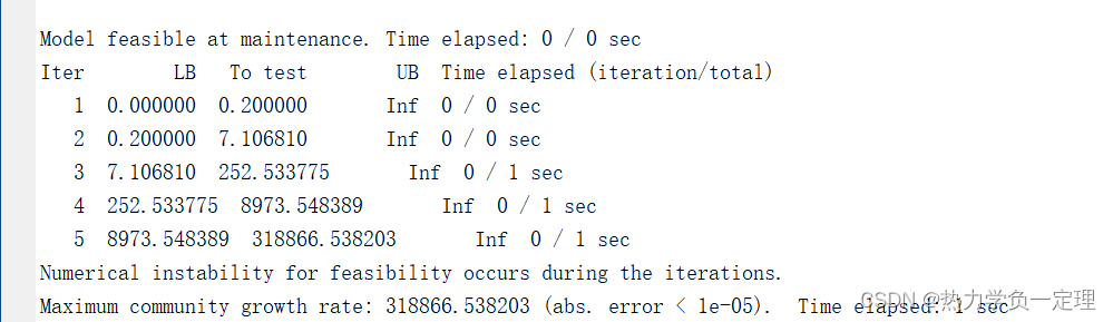
% SteadyCom in general can be finished within 20 iterations, i.e. solving 20
% LPs (usually faster if using Matlab |fzero|) for an accuracy of 1e-6 for the
% maximum community growth rate. The actual computation time depends on the size
% of the community metabolic network. The current |EcCom| model has 6971 metabolites
% and 9831 reactions. It took 18 seconds for a MacBook Pro with 2.5 GHz Intel
% Core i5, 4 GB memory running Matlab R2016b and Cplex 12.7.1.
%
% Since the FVA and POA analysis can be time-consuming for large models with
% a large number of reactions to be analyzed, SteadyComFVA and SteadyComPOA support
% parrallelization using the Matlab Distributed Computing Toolbox (|parfor| for
% SteadyComFVA and |spmd| for SteadyComPOA).
%
% Test SteadyComFVA with 2 threads:
%%
options.rxnNameList = EcCom.rxns(1:100); % test FVA for the first 50 reactions
options.optGRpercent = 99;
options.algorithm = 1;
options.threads = 1; % test single-thread computation first
options.verbFlag = 0; % no verbose output
tic;
[minF1, maxF1] = SteadyComFVA(EcCom, options);
t1 = toc;
if isempty(gcp('nocreate'))
parpool(2); % start a parallel pool
end
options.threads = 2; % two threads (0 to use all available workers)
tic;
[minF2, maxF2] = SteadyComFVA(EcCom, options); % test single-thread computation first
t2 = toc;
fprintf('Maximum difference between the two solutions: %.4e\n', max(max(abs(minF1 - minF2)), max(abs(maxF1 - maxF2))));
fprintf('\nSingle-thread computation: %.0f sec\nTwo-thread computation: %.0f sec\n', t1, t2);
%%
% If there are many reactions to be analyzed, use |options.saveFVA| to give
% a relative path for saving the intermediate results. Even though the computation
% is interrupted, by calling |SteadyComFVA| with the same |options.saveFVA|, the
% program will detect previously saved results and continued from there.
%
% Test SteadyComPOA with 2 threads:
options.rxnNameList = EcCom.rxns(find(abs(result.flux) > 1e-2, 6));
options.savePOA = 'POA/EcComParallel'; % save with a new name
options.verbFlag = 3;
options.threads = 2;
options.Nstep = 5; % use a smaller number of steps for test
tic;
[POAtable1, fluxRange1] = SteadyComPOA(EcCom, options);
t3 = toc;
%%
% The parallelization code uses |spmd| and will redistribute jobs once any
% of the workers has finished to maximize the computational efficiency.
options.savePOA = 'POA/EcComSingeThread';
options.threads = 1;
tic;
[POAtable2, fluxRange2] = SteadyComPOA(EcCom, options);
t4 = toc;
dev = 0;
for i = 1:size(POAtable1, 1)
for j = i:size(POAtable1, 2)
dev = max(max(max(abs(POAtable1{i, j} - POAtable2{i, j}))));
dev = max(dev, max(max(abs(fluxRange1 - fluxRange2))));
end
end
fprintf('Maximum difference between the two solutions: %.4e\n', dev);
fprintf('\nSingle-thread computation: %.0f sec\nTwo-thread computation: %.0f sec\n', t4, t3);
%%
% The advantage will be more significant for more targets to analyzed and
% more threads used. Similar to |SteadyComFVA|, |SteadyComPOA| also supports continuation
% from previously interrupted computation by calling with the same |options.savePOA|.
%
%
%% REFERENCES
% _[1] _Chan SHJ, Simons MN, Maranas CD (2017) SteadyCom: Predicting microbial
% abundances while ensuring community stability. PLoS Comput Biol 13(5): e1005539.
% https://doi.org/10.1371/journal.pcbi.1005539
%
% _[2] _Khandelwal RA, Olivier BG, Röling WFM, Teusink B, Bruggeman FJ (2013)
% Community Flux Balance Analysis for Microbial Consortia at Balanced Growth.
% PLoS ONE 8(5): e64567. https://doi.org/10.1371/journal.pone.0064567
%
% __
4. 结果展示
6. 代码注释
%清理环境变量
% clc
% clear
%初始环境(只一次运行后执行,更新环节)
%initCobraToolbox;
%读取模型
% 模型测试时候优先把每个模型单独构建群落模型,修改生物量的表示方式并重新保存
modelFileName_1='AF.xls';
modelFileName_2='AP.xls';
modelFileName_3='AT.xls';
modelFileName_4='LB.xls';
models1= readCbModel(modelFileName_1);
models2= readCbModel(modelFileName_2);
models3= readCbModel(modelFileName_3);
models4= readCbModel(modelFileName_4);
models{1,1} = models1;
models{2,1} = models2;
models{3,1} = models3;
models{4,1} = models4;
%测试
XP1=models1;
JY4=models4;
modelss{1,1} = XP1;
modelss{2,1} = JY4;
%要求模型中生物量反应的标识为 bio 且反应中包含关键的代谢物 每个代谢物能够合并
%构建多菌的群落模型
[modelJoint] = createMultipleSpeciesModel(models);
%获取群落代谢信息
nameTagsModels={'model1','model2','model3','model4'};%物种反应名称前缀
[modelJoint.infoCom,modelJoint.indCom]=getMultiSpeciesModelId(modelJoint,nameTagsModels);
%生物量转换的标记位置 生物量产生计算
%spBm=[990,1834];
% spBm=zeros(size(nameTagsModels));
for i=1:size(nameTagsModels,2)
spBm(1,i)=find(strncmp(modelJoint.rxns, strcat(nameTagsModels(i),'_biomass'), 10));
spBm1(1,i)=strcat(nameTagsModels(i),'_biomass')
end
modelJoint.indCom.spBm=spBm;
modelJoint.infoCom.spBm=spBm1;
% modelJoint.infoCom=modelJoint.indCom;
%分析群落模型的相互作用
%改变所有物质上限
modelJoint.ub(modelJoint.indCom.EXsp(:)~=0) = 1000;
%展示模型上下限
printUptakeBoundCom(modelJoint, 1);
% 选项
%生长速率拟合,第一个菌的生长速率为0.1 第二个菌为0.2
% options.GRfx = [1,0.1;2,0.3];
% %判断是否生长
% options.feasCrit=1;
% options.GRguess=[0.2,0.8];
options = struct();
options.GRguess = 0.1; % initial guess for max. growth rate 初始生长速率
options.GRtol = 1e-6; % tolerance for final growth rate
options.algorithm = 1; % use the default algorithm (simple guessing for bounds, followed by matlab fzero)
options.algorithm = 2; % use the simple guessing algorithm
options.guessMethod=1;
% options.BMcon=[100;100;100;50];
% options.BMgdw=[1;2;1;2];
[sol, result, LP, LPminNorm, indLP] =SteadyCom(modelJoint,options);
[sol, result, LP, LPminNorm, indLP] =SteadyCom(modelJoint);
%%
options.optBMpercent = 100;
n = size(modelJoint.S, 2); % number of reactions in the model
% options.rxnNameList is the list of reactions subject to FVA. Can be reaction names or indices.
% Use n + j for the biomass variable of the j-th organism. Alternatively, use {'X_j'}
% for biomass variable of the j-th organism or {'X_Ec1'} for Ec1 (the abbreviation in EcCom.infoCom.spAbbr)
options.rxnNameList = spBm1;
options.optGRpercent = [1:10:99, 0:10:100]; % perform FVA at various percentages of the maximum growth rate, 89, 89.1, 89.2, ..., 100
[fvaComMin,fvaComMax] = SteadyComFVA(modelJoint, options);
[minFlux, maxFlux, minFD, maxFD, GRvector, result, LP] = SteadyComFVA(modelJoint);
%%
%修改目标函数
modelJoint = changeObjective(modelJoint,{'model1_biomass','model2_biomass','model3_biomass'},3); %求解的产物
%sol = optimizeCbModel(modelCom,'max','one');%求解目标产物的最大转换率,设置求解参数,
[POAtable, fluxRange, Stat, GRvector] = SteadyComPOA(modelJoint);
% [sol, result, LP, LPminNorm, indLP] = SteadyComCplex(modelJoint);
%% 测试单个模型
modelCom = changeObjective(modelJoint,{'model1_biomass','model2_biomass','model3_biomass'},3); %求解的产物,设定需要观察的目标产物, M11_4为底物编号
modelCom = changeObjective(modelJoint,{'model1_biomass'},1);
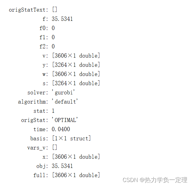
sol = optimizeCbModel(modelJoint,'max','one');%求解目标产物的最大转换率,设置求解参数,
sol.obj=sol.f;


 4399
4399

 被折叠的 条评论
为什么被折叠?
被折叠的 条评论
为什么被折叠?
 到【灌水乐园】发言


