


前言
灰度,可以理解为图像经过灰度处理后的像素值。我们可以通过对图像灰度做一些调整,以达到不同的效果,比如是图片变亮、对比度增强等。
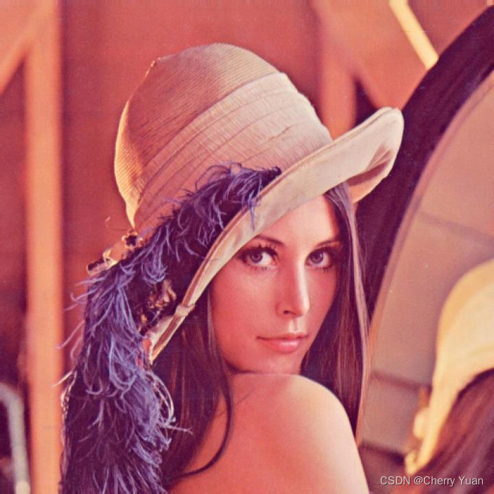
导入原图
from PIL import Image
import numpy as np
import matplotlib.pyplot as plt
#打开图像(numpy不具备打开图像的功能,只能通过其他的库,比如pillow或者opencv,返回的是图片格式、图片颜色模式、图片宽高、图片在内存中的地址)
img = Image.open("example.jpg")
# print(img)

#获取图像的尺寸(pillow库的Image获取的图像数据是PIL格式的,但可以通过size获取图像的宽和高,并不能获取到图像第三维度的RGB通道数据)
size = img.size
# print(size)

#获取图像的宽和高
width,height = img.size

#numpy获取图像的形状(高、宽、RGB三通道数据:Height,Width,···),先要将图像的PIL格式数据转化为numpy的ndarray类型数据。
image_1 = np.array(img)
# print(image_1)
shape = image_1.shape
# print(shape)

#加载图像(此处的加载属于pillow中的方法,获取的是PIL格式的图像在内存中的地址)
img_1 = img.load()
# print(img_1)

#获取图像某一像素点的灰度值
gray_value = img_1[0,0]
# print(gray_value)

#新建numpy类型的数组,初始元素全为0,numpy.zeros()内部存放的元素,是一个,要么是单个整型数据,要么一个元组表示的图像形状。
image = np.zeros((height,width,3))
# print(image)
线性变换
#线性变换,方法一:修改图片numpy数据,灰度线性变换加权公式:GRAY = 0.3 * R + 0.59 * G + 0.11 * B
for i in range(width):
    for j in range(height):
        image[i][j] = image_1[i][j][0] * 0.3 + image_1[i][j][1] * 0.59 + image_1[i][j][2] * 0.11

#调整图像numpy数组的格式,在图像处理中,Unit8数据类型被用来表示像素的灰度值。
#灰度值是指像素的亮度,它的取值范围是0~255,其中0表示黑色,255表示白色。
#在图像处理中,我们可以通过改变像素的灰度值来实现图像的亮度、对比度、色彩等方面的调整。
image = image.astype(np.uint8)

# 将numpy数组转换为PIL图像
image_2 = Image.fromarray(image)

image_2.show()
#线性变换,方法二:修改图片numpy数据,灰度线性变换加权公式:GRAY = 0.3 * R + 0.59 * G + 0.11 * B
image_3 = image_1[:,:,0] * 0.3 + image_1[:,:,1] * 0.59 + image_1[:,:,2] * 0.11

image_3 = image_3.astype(np.uint8)

plt.imshow(image_3,cmap='gray') # plt默认显示三个通道,设置cmap='gray'显示一个通道
<matplotlib.image.AxesImage at 0x23682718648>
#线性变换,方法二:修改图片numpy数据,灰度线性变换加权公式:GRAY = 0.299 * R + 0.587 * G + 0.114 * B
image_4 = image_1[:,:,0] * 0.299 + image_1[:,:,1] * 0.587 + image_1[:,:,2] * 0.114

image_4 = image_4.astype(np.uint8)

# 将numpy数组转换为PIL图像
image_4 = Image.fromarray(image_4)

image_4.show()
图像反转
以上的我们称之为恒等变换,除开RGB三通道像素值前面的系数,它们各自的幂数都是1。
另外,线性变换里面还有一个特例,也就是图像反转
图像反转(Invert)是针对图像的像素值,即颜色的逆转,而像素的位置不变。
图像翻转(Flip)是沿对称轴的几何变换,像素值不变。
图像反转(公式为s = L - 1 - r,其中r和s分别代表图像处理前后的像素值,它们所处的灰度级区间是[0,L-1]。
s
=
L
−
1
−
r
,
r
∈
[
0
,
L
−
1
]
,
s
∈
[
0
,
L
−
1
]
s=L-1-r,r \in[0,L-1],s \in[0,L-1]
s=L−1−r,r∈[0,L−1],s∈[0,L−1]
from PIL import Image
import numpy as np
import matplotlib.pyplot as plt
#打开图像(numpy不具备打开图像的功能,只能通过其他的库,比如pillow或者opencv,返回的是图片格式、图片颜色模式、图片宽高、图片在内存中的地址)
img = Image.open("example.jpg")
#pillow里的convert()函数内部参数分别是mode、matrix、dither、palette、colors,我们此处只用第一个mode
#mode = "L",表示的是图片转化为灰度图,转换公式就是:GRAY = 0.299 * R + 0.587 * G + 0.114 * B。
#mode = "RGB",通常是对彩色图片进行加强3x8位像素,真彩色
#mode = "YCbCr",3x8位像素,彩色视频格式
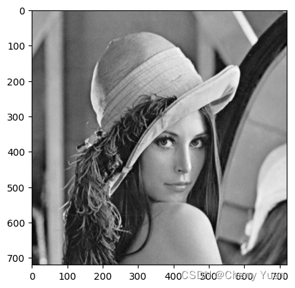
gray_image = img.convert('L')
gray_img = np.array(gray_image)
# print(gray_img)
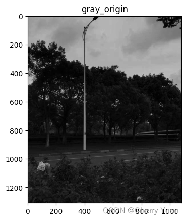
plt.title("gray_origin")
#plt.imshow()显示图片,cmap默认值是viridis(翠绿色),因此用plt显示图片是,需要把cmap值置为“gray”。
#当然,如果用PIL结合numpy显示图片则不用转化。
plt.imshow(gray_img,cmap='gray')
plt.show()
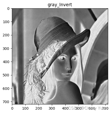
#图像反转,选用的灰度区间是[0,255],一共256各灰度等级。
width,height = gray_img.shape #获取图像形状,宽和高
img_new = np.ones((width,height)) #新建全一矩阵(数组)
img_256 = img_new * 255 #新建元素全是255的矩阵,形状和原图一致。
gray_invert = img_256 - gray_img[:,:]
# print(gray_invert)
plt.title("gray_Invert")
plt.imshow(gray_invert,cmap='gray')
plt.show()

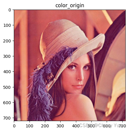
#当然我们还可以对彩色图进行图像反转

img_color = np.array(img)

plt.title("color_origin")
plt.imshow(img_color,cmap='brg')
plt.show()

width,height,_ = img_color.shape  #获取图像形状,宽和高
img_new_1 = np.ones((width,height,3))  #新建全一矩阵(数组)
img_256_1 = img_new_1 * 255      #新建元素全是255的矩阵,形状和原图一致。
color_invert = img_256_1 - img_color[:,:,:]
# print(color_invert)

plt.title("color_Invert")
plt.imshow(color_invert,cmap='brg')
plt.show()

非线性变换——对数变换
非线性变换是指运用非线性函数调整原始图像的灰度范围,常用方法有灰度变换和幂律变换。
注意:非线性灰度变换在运算过程中,像素值要暗示书来计算,计算结果也是实数,要注意图像数据类型的转换。
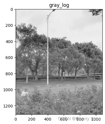
对数变换是指将输入范围变窄的地灰度级映射为范围较宽的灰度级。是较暗区域的对比度增强,提升图像的暗部细节。公式如下:
s
=
c
∗
log
(
1
+
r
)
s = c * \log(1 + r)
s=c∗log(1+r)
#对数变换公式如上,其中c是比例系数,r、s分别对应原视图像和变换图像的灰度值。
#对数变换实现了扩展低灰度级而压缩高灰度级的效果。

#灰度图对数变换
from PIL import Image
import numpy as np
import matplotlib.pyplot as plt

img = Image.open("example_1.jpg")


gray_image = img.convert('L')
gray_img = np.array(gray_image)

plt.title("gray_origin")
plt.imshow(gray_img,cmap='gray')
plt.show()

c = 1
gray_log = c*np.log(1 + gray_img[:,:])
# print(gray_log)

plt.title("gray_log")
plt.imshow(gray_log,cmap='gray')
plt.show()

[[4.395 4.395 4.395 ... 2.834 2.773 2.709]
 [4.395 4.395 4.395 ... 1.946 2.303 2.639]
 [4.395 4.395 4.395 ... 2.639 2.834 3.295]
 ...
 [3.258 3.135 3.045 ... 2.303 2.303 2.303]
 [3.178 3.135 3.045 ... 2.303 2.303 2.303]
 [3.135 3.092 3.045 ... 2.398 2.398 2.398]]
非线性变换——幂律变换
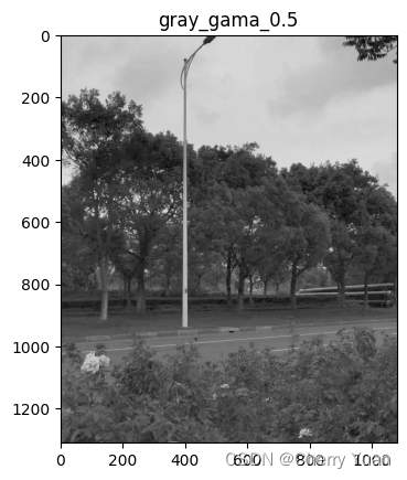
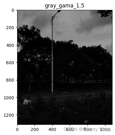
幂律变换,又称伽马变换,或指数变换。它可以提升暗部细节,对曝光过度或过暗的图片进行矫正。公式如下:
s = c r γ , γ > 0 s = cr^\gamma,\gamma > 0 s=crγ,γ>0
其中r和s分别代表原始图像和变换图像的灰度值, Γ \Gamma Γ是伽马系数,c是比例系数。
当$ 0<\Gamma<1 $时,拉伸了图像的低灰度级,压缩了图像的高灰度级,降低了图像的对比度。
当 Γ > 1 \Gamma>1 Γ>1时,拉伸了图像高灰度级,压缩了图像的低灰度级,在增强了图像的对比度。
有时,为了显示校准的图像,也会在幂律变换的公式中加上偏移: s = c ( r + ϵ ) γ s = c(r + \epsilon)^\gamma s=c(r+ϵ)γ。
#灰度图幂律变换
from PIL import Image
import numpy as np
import matplotlib.pyplot as plt

img = Image.open("example_1.jpg")


gray_image = img.convert('L')
gray_img = np.array(gray_image)

plt.title("gray_origin")
plt.imshow(gray_img,cmap='gray')
plt.show()

#此处我们将c置为1
c = 1

'''伽马值为0.5的情况'''
gama = 0.5
gray_gama_half = c*(gray_img[:,:] ** gama)
# print(gray_log)

plt.title("gray_gama_0.5")
plt.imshow(gray_gama_half,cmap='gray')
plt.show()


'''伽马值为1.5的情况'''
gama = 1.5
gray_gama_one_and_half = c*(gray_img[:,:] ** gama)
# print(gray_log)

plt.title("gray_gama_1.5")
plt.imshow(gray_gama_one_and_half,cmap='gray')
plt.show()

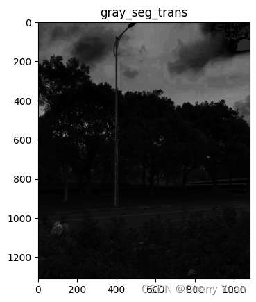
分段线性变换
分段线性变换。优点是形式可以是任意的,即自定义部分灰度级范围内的图像改变对比度。缺点是参数太多了,不易确定。公式如下:
s
=
{
s
1
r
1
∗
r
,
0
≤
r
<
r
1
s
2
−
s
1
r
2
−
r
1
∗
(
r
−
r
1
)
,
r
1
≤
r
<
r
2
L
−
s
1
L
−
r
1
∗
(
r
−
r
2
)
,
r
2
≤
r
<
L
s=\begin{cases} \frac{s_1}{r_1}*r,0 \leq r<r_1\\ \frac{s_2-s_1}{r_2-r_1}*(r-r_1),r_1 \leq r<r_2\\ \frac{L-s_1}{L-r_1}*(r-r_2),r_2 \leq r<L \end{cases}
s=⎩
⎨
⎧r1s1∗r,0≤r<r1r2−r1s2−s1∗(r−r1),r1≤r<r2L−r1L−s1∗(r−r2),r2≤r<L
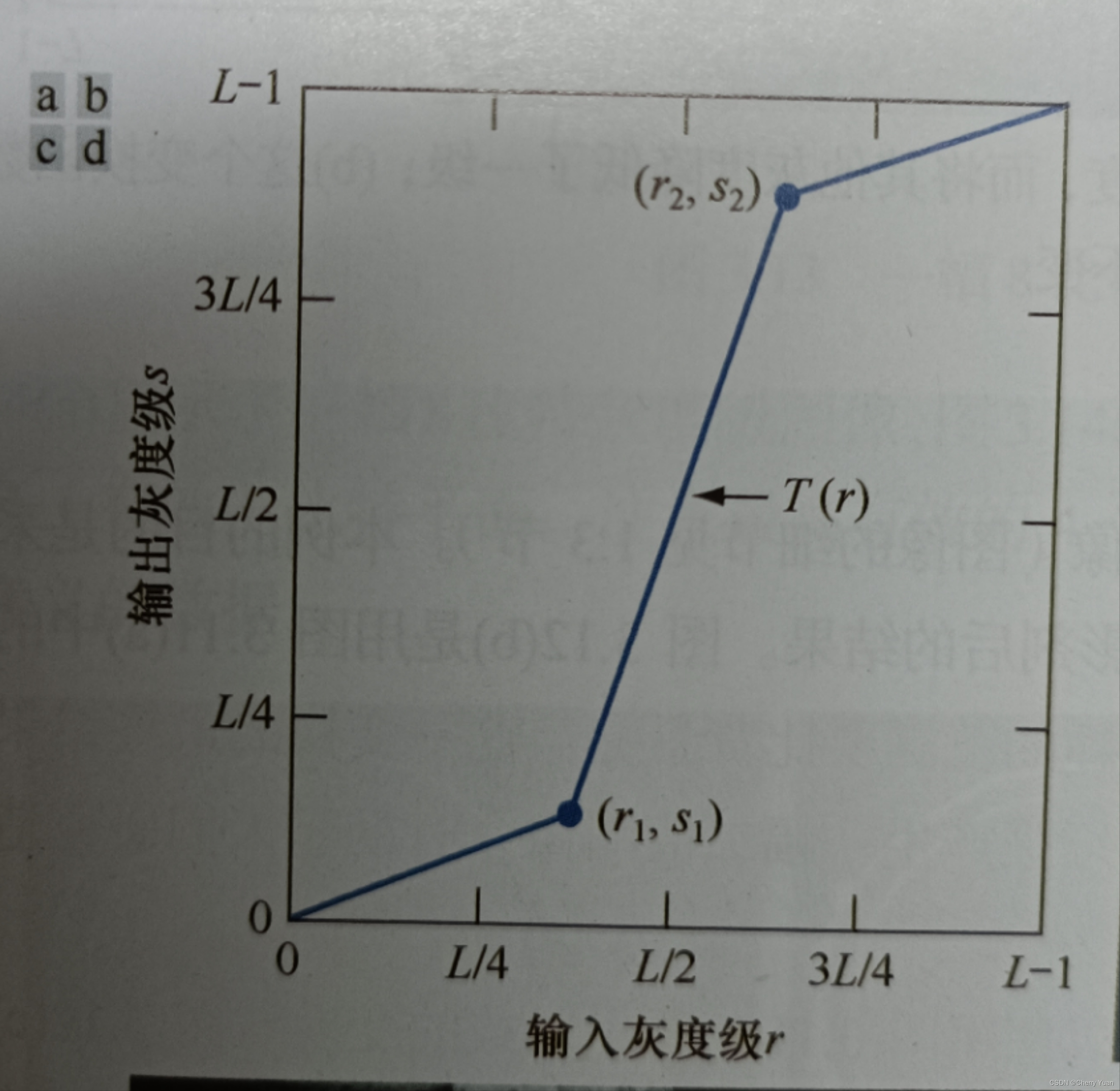
其中r和s分别代表原始图像和变换图像的灰度值。我们正常实验中遇到的灰度级最大值L一般为255,r、r1、r2、s、s1、s2的取值范围均是[0,255]。
如图,若r1=r2,s1=s2,把么变换就是一个不改变灰度的线性函数 y = x。
若r1=r2,s1=0,s=L-1,那么变换就是一个二值图像处理的函数。
#分段线性变换
from PIL import Image
import numpy as np
import matplotlib.pyplot as plt

img = Image.open("example_1.jpg")


gray_image = img.convert('L')
gray_img = np.array(gray_image)

#获取图像的宽高
width,height = gray_img.shape  #获取图像形状,宽和高

plt.title("gray_origin")
plt.imshow(gray_img,cmap='gray')
plt.show()

#预设几个参数的值
r1,s1 = 64,32
r2,s2 = 128,224
L = 255

#创建一个形状和原图相同的数组
gray_seg_trans = np.empty([width,height])

for i in range(width):
    for j in range(height):
        if gray_img[i,j] < r1:
            gray_seg_trans[i,j] = (s1/r1) * gray_img[i,j]
        elif gray_img[i,j] >= r1 and gray_img[i,j] < r2:
            gray_seg_trans[i,j] = ((s2-s1)/(r2-r1)) * (gray_img[i,j] - r1)
        else:
            gray_seg_trans[i,j] = ((L-s2)/(L-r2)) * (gray_img[i,j] - r2)


plt.title("gray_seg_trans")
plt.imshow(gray_seg_trans,cmap='gray')
plt.show()
'''此处设置的参数效果是增强了对比度'''
结语
以上几种灰度变换的原理参考冈萨雷斯的《数字图像处理》第四版,若诸位有什么需要补充的,也可以在评论区积极留言,互相学习!


 2000
2000


 被折叠的 条评论
为什么被折叠?
被折叠的 条评论
为什么被折叠?
 到【灌水乐园】发言


