机器学习笔记之生成模型综述(一)生成模型介绍

引言

从本节开始，将介绍生成模型的相关概念。

生成模型介绍

生成模型，单从名字角度，可以将其认识为：生成样本的模型。从流程的角度，它可以理解为：

• 给定一个数据集合，基于该数据集合进行建模，并通过数据集合学习出模型的参数信息；
• 根据已学习出的参数信息，使用模型构建出新的数据。

但生成新的数据仅是生成模型的一个任务/目标，通过生成新数据的模型对生成模型进行判别可能是很片面的。

例如之前介绍的高斯混合模型($\text{Gaussain Mixture Model,GMM}$)，它的概率图结构可表示为：

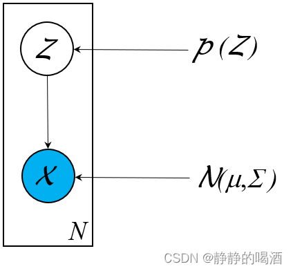
其中$\mathcal{Z}$是一个一维、离散型随机变量，对应的$\mathcal{X}\mid \mathcal{Z}$服从高斯分布：
Z ∼ Discrete Distribution ( 1 , 2 , ⋯   , K ) X ∣ Z ∼ N ( μ k , Σ k ) k ∈ { 1 , 2 , ⋯   , K } \begin{aligned} \mathcal Z & \sim \text{Discrete Distribution}(1,2,\cdots,\mathcal K) \\ \mathcal X \mid \mathcal Z & \sim \mathcal N(\mu_{k},\Sigma_k) \quad k \in \{1,2,\cdots,\mathcal K\} \end{aligned} ZX∣Z​∼Discrete Distribution(1,2,⋯,K)∼N(μk​,Σk​)k∈{1,2,⋯,K}​
只要能够确定隐变量$\mathcal{Z}$的概率分布${\mathcal{P}}_{\mathcal{Z}}$，以及高斯分布参数$({\mu }_{\mathcal{Z}},{\Sigma }_{\mathcal{Z}})$，就可以从概率模型中源源不断生成出样本：
这里${\mu }_{\mathcal{Z}},{\Sigma }_{\mathcal{Z}},{\mathcal{P}}_{\mathcal{Z}}$均表示模型参数。
$$\{\begin{array}{l}\forall z^{(i)}\in \mathcal{Z}\\ z^{(i)}\sim {\mathcal{P}}_{z^{(i)}}\\ x^{(i)}\mid z^{(i)}\sim \mathcal{N}({\mu }_{z^{(i)}},{\Sigma }_{z^{(i)}})\end{array}$$
不可否认的是，高斯混合模型就是一个生成模型。它所处理的任务主要是无监督的聚类任务。
相反，监督学习中，是否也存在生成模型呢？例如：朴素贝叶斯分类器(Naive Bayes Classifier)，它的概率图结构表示如下：

这是一个基于朴素贝叶斯假设的分类模型：
文字描述是：在标签$\mathcal{Y}$确定的条件下，随机变量集合$\mathcal{X}$内各随机变量相互独立。$p$表示$\mathcal{X}$内随机变量的数量；$k$表示随机变量$\mathcal{Y}$划分类的数量。
x i ⊥ x j ∣ Y = l { i , j ∈ { 1 , 2 , ⋯   , p } i ≠ j l ∈ { 1 , 2 , ⋯   , k } x_i \perp x_j \mid \mathcal Y=l \quad \begin{cases} i,j \in \{1,2,\cdots,p\} \\ i \neq j \\ l \in \{1,2,\cdots,k\} \end{cases} xi​⊥xj​∣Y=l⎩ ⎨ ⎧​i,j∈{1,2,⋯,p}i=jl∈{1,2,⋯,k}​
关于$\mathcal{P}(\mathcal{X}\mid \mathcal{Y})$可表示为：
$$\mathcal{P}(\mathcal{X}\mid \mathcal{Y})=\prod _{i=1}^p\mathcal{P}(x_i\mid \mathcal{Y})$$
在分类过程中，通过软分类对$\mathcal{Y}$的后验概率进行判别，并进行分类：
将后验概率$\mathcal{P}(\mathcal{Y}\mid \mathcal{X})$通过贝叶斯定理转化为似然$\mathcal{P}(\mathcal{X}\mid \mathcal{Y})$ × 先验概率$\mathcal{P}(\mathcal{Y})$的形式。
$$\begin{array}{rl}\mathcal{P}(\mathcal{Y}=m\mid \mathcal{X})& \stackrel{\text{?}}{\iff }\mathcal{P}(\mathcal{Y}=n\mid \mathcal{X})\\ \propto \mathcal{P}(\mathcal{X}\mid \mathcal{Y}=m)\cdot \mathcal{P}(\mathcal{Y}=m)& \stackrel{\text{?}}{\iff }\mathcal{P}(\mathcal{X}\mid \mathcal{Y}=n)\cdot \mathcal{P}(\mathcal{Y}=n)\end{array}$$
显然，我们也无法从监督/无监督的角度对生成模型进行定义。再举一个例子：逻辑回归(Logistic Regression)，虽然它和朴素贝叶斯分类器一样，也是软分类的经典算法，但它不是生成模型。因为它的核心是 通过$\text{Sigmoid,Softmax}$函数直接对标签$\mathcal{Y}$的后验概率进行比较：
这里以二分类为例，对应的是$\text{Sigmoid}$函数。
$$\begin{array}{rl}& \{\begin{array}{l}\mathcal{P}(\mathcal{Y}=1\mid \mathcal{X})=\text{Sigmoid}({\mathcal{W}}^T\mathcal{X}+b)\\ \mathcal{P}(\mathcal{Y}=0\mid \mathcal{X})=1-\text{Sigmoid}({\mathcal{W}}^T\mathcal{X}+b)\end{array}\\ & \mathcal{P}(\mathcal{Y}=1\mid \mathcal{X})\stackrel{\text{?}}{\iff }\mathcal{P}(\mathcal{Y}=0\mid \mathcal{X})\end{array}$$
从这里可以看出朴素贝叶斯分类器与逻辑回归的差别：

• 关于逻辑回归，直接对条件概率$\mathcal{P}(\mathcal{Y}\mid \mathcal{X})$进行建模，也就是说，逻辑回归中只关注$\text{Sigmoid}$函数的返回结果，对$\mathcal{X}$的特征并不关心；
• 相反，朴素贝叶斯分类器不仅没有直接比较$\mathcal{P}(\mathcal{Y}\mid \mathcal{X})$，而是通过贝叶斯定理转化成$\mathcal{P}(\mathcal{X}\mid \mathcal{Y})\cdot \mathcal{P}(\mathcal{Y})$进行比较。并且它对$\mathcal{X}$的特征提出了严苛的条件独立性假设。

综上，生成模型的关注点均在样本分布本身，并根据样本分布的特点进行建模。和具体的任务之间没有具体关联关系：

• 如果是包含标签信息$\mathcal{Y}$的监督学习任务，如朴素贝叶斯分类器。直接对$\mathcal{P}(\mathcal{X},\mathcal{Y})$进行建模：
  $$\begin{array}{rl}\mathcal{P}(\mathcal{Y}\mid \mathcal{X})=\frac{\mathcal{P}(\mathcal{X},\mathcal{Y})}{\mathcal{P}(\mathcal{X})}\propto \mathcal{P}(\mathcal{X},\mathcal{Y})& =\mathcal{P}(\mathcal{X}\mid \mathcal{Y})\cdot \mathcal{P}(\mathcal{Y})\\ \mathcal{P}(\mathcal{X}\mid \mathcal{Y}=m)\cdot \mathcal{P}(\mathcal{Y}=m)& \stackrel{\text{?}}{\iff }\mathcal{P}(\mathcal{X}\mid \mathcal{Y}=n)\cdot \mathcal{P}(\mathcal{Y}=n)\end{array}$$

• 如果是无监督学习任务，如隐变量模型($\text{Latent Variable Model,LVM}$)，可以通过构造隐变量$\mathcal{Z}$，通过对$\mathcal{P}(\mathcal{X},\mathcal{Z})$进行建模。

  • 在无监督模型中，这种思想更加深刻。由于至始至终仅有样本特征是我们能够观测到的已知信息。无论是隐变量，还是模型，都是基于样本特征的性质构建的合理假设。
  • 当然，针对无监督学习任务，不是仅有隐变量模型一种选择。如‘自回归模型’(AutoRegressive,AR),它就是一种直接对$\mathcal{P}(\mathcal{X})$建模的方法。

  如：玻尔兹曼机系列的能量模型：
  其中$v$表示观测变量；$h$表示隐变量。
  P ( v , h ) = 1 Z exp ⁡ { − E [ v , h ] } \begin{aligned} \mathcal P(v,h) = \frac{1}{\mathcal Z} \exp \{-\mathbb E[v,h]\} \end{aligned} P(v,h)=Z1​exp{−E[v,h]}​
  如高斯混合模型：
  $$\begin{array}{rl}\mathcal{P}(\mathcal{X})& =\sum _{\mathcal{Z}}\mathcal{P}(\mathcal{X},\mathcal{Z})\\ & =\sum _{\mathcal{Z}}\mathcal{P}(\mathcal{X}\mid \mathcal{Z})\cdot \mathcal{P}(\mathcal{Z})\\ & =\sum _{k=1}^{\mathcal{K}}{p}_k\cdot \mathcal{N}({\mu }_k,{\Sigma }_k)\sum _{k=1}^{\mathcal{K}}{p}_k=1\end{array}$$

通常也称生成模型为概率生成模型。
生成对抗网络中的样本生成过程表示为$x=\mathcal{G}(\mathcal{Z};{\theta }_{gene})$,其中$\mathcal{Z}$是一个简单分布。虽然这里$\mathcal{G}(\mathcal{Z};{\theta }_{gene})$是一个由前馈神经网络构成的计算图，但它依然描述的是样本自身的概率模型/概率分布。因此，生成对抗网络是一个概率生成模型。

下一节将从监督与无监督的角度介绍现阶段经典的概率模型。

相关参考：
生成模型1-定义