


Numpy应用案例
注:使用numpy库来对图像进行处理。这里我们使用matplotlib.pyplot的相关方法来辅助。
import numpy as np
import matplotlib.pyplot as plt
图像读取与显示
- plt.imread:读取图像,返回图像的数组。
- plt.imshow:显示图像。
- plt.imsave:保存图像。
说明:
- imread方法默认只能处理png格式的图像,如果需要处理其他格式的图像,需要安装pillow库。
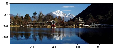
# 读取图像,返回图像的数组
a = plt.imread("1.png")
print(type(a))
print(a.shape)
a
<class 'numpy.ndarray'>
(360, 920, 3)


array([[[0.36862746, 0.6156863 , 0.827451  ],
        [0.35686275, 0.6039216 , 0.8156863 ],
        [0.35686275, 0.6039216 , 0.8156863 ],
        ...,
        [0.00784314, 0.00392157, 0.02745098],
        [0.00784314, 0.00392157, 0.02745098],
        [0.01176471, 0.00784314, 0.03137255]],

       [[0.36862746, 0.6156863 , 0.827451  ],
        [0.35686275, 0.6039216 , 0.8156863 ],
        [0.35686275, 0.6039216 , 0.8156863 ],
        ...,
        [0.00784314, 0.00392157, 0.02745098],
        [0.00784314, 0.00392157, 0.02745098],
        [0.01176471, 0.00784314, 0.03137255]],

       [[0.36862746, 0.6156863 , 0.8235294 ],
        [0.35686275, 0.6039216 , 0.8117647 ],
        [0.35686275, 0.6039216 , 0.8117647 ],
        ...,
        [0.00784314, 0.00392157, 0.02745098],
        [0.01176471, 0.00784314, 0.03137255],
        [0.01176471, 0.00784314, 0.03137255]],

       ...,

       [[0.14117648, 0.34901962, 0.56078434],
        [0.14117648, 0.34901962, 0.56078434],
        [0.13725491, 0.34509805, 0.5568628 ],
        ...,
        [0.00392157, 0.00392157, 0.00392157],
        [0.00392157, 0.00392157, 0.00392157],
        [0.00392157, 0.00392157, 0.00392157]],

       [[0.14509805, 0.3529412 , 0.5647059 ],
        [0.14117648, 0.34901962, 0.56078434],
        [0.13725491, 0.34509805, 0.5568628 ],
        ...,
        [0.00392157, 0.00392157, 0.00392157],
        [0.00392157, 0.00392157, 0.00392157],
        [0.00392157, 0.00392157, 0.00392157]],

       [[0.14509805, 0.3529412 , 0.5647059 ],
        [0.14117648, 0.34901962, 0.56078434],
        [0.13725491, 0.34509805, 0.5568628 ],
        ...,
        [0.00392157, 0.00392157, 0.00392157],
        [0.00392157, 0.00392157, 0.00392157],
        [0.00392157, 0.00392157, 0.00392157]]], dtype=float32)
# 显示图像
plt.imshow(a)
<matplotlib.image.AxesImage at 0x1596120b2b0>
![[外链图片转存失败,源站可能有防盗链机制,建议将图片保存下来直接上传(img-i3Mr5eCq-1577161964516)(output_4_1.png)]](https://img-blog.csdnimg.cn/20191224123557347.png)
# 保存图片
plt.imsave("1_1.png",a)
显示纯色图像
- 显示白色图像
- 显示黑色图像
- 显示指定颜色图像
# 图像可以有两种表示方式。一种是使用无符号的np.uint8,取值为0~255。一种是使用float类型表示,取值为0.0~1.0。
# 其中,float值的0.0对应整数类型的0,float类型的1.0对应整数类型的255。
# int8  (-2**7到2**7-1)   uint(0-2**8-1)  无符号的不用表示符号位,所以多出一位
x = np.ones(shape=(100, 100, 3))  # 数组元素全为1.0 对应 255
# 显示纯白色图像
plt.imshow(x)
<matplotlib.image.AxesImage at 0x15961668860>

# 显示纯黑色图像
x = np.zeros((100, 100, 3))
plt.imshow(x)
<matplotlib.image.AxesImage at 0x159616c36a0>
# 使用整数unint8类型来显示。
x = np.full(shape=(100, 100, 3), fill_value=255, dtype=np.uint8)
plt.imshow(x)
<matplotlib.image.AxesImage at 0x1596171d518>
# 显示纯色(228, 238, 249)
x = np.full(shape=(100, 100, 3), fill_value=1, dtype=np.uint8)
# 注意,修改数组x最低维的元素,不能这样操作。
# 因为这样做没有修改x的元素,而是令x解绑,去绑定了新的对象。
# x = [228, 238, 249]
# x[:] = [228, 238, 249]  会进行广播操作等价于 x[:,:] = [228, 238, 249]
x[:,:] = [228, 238, 249]
print(x)
plt.imshow(x)
[[[228 238 249]
  [228 238 249]
  [228 238 249]
  ...
  [228 238 249]
  [228 238 249]
  [228 238 249]]

 [[228 238 249]
  [228 238 249]
  [228 238 249]
  ...
  [228 238 249]
  [228 238 249]
  [228 238 249]]

 [[228 238 249]
  [228 238 249]
  [228 238 249]
  ...
  [228 238 249]
  [228 238 249]
  [228 238 249]]

 ...

 [[228 238 249]
  [228 238 249]
  [228 238 249]
  ...
  [228 238 249]
  [228 238 249]
  [228 238 249]]

 [[228 238 249]
  [228 238 249]
  [228 238 249]
  ...
  [228 238 249]
  [228 238 249]
  [228 238 249]]

 [[228 238 249]
  [228 238 249]
  [228 238 249]
  ...
  [228 238 249]
  [228 238 249]
  [228 238 249]]]


<matplotlib.image.AxesImage at 0x1596176deb8>
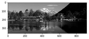
转换为灰度图
灰度图的数据可以看成是二维数组,元素取值为0 ~ 255,其中,0为黑色,255为白色。从0到255逐渐由暗色变为亮色。
灰度图转换(ITU-R 601-2亮度变换):
L = R * 299 / 1000 + G * 587 / 1000 + B * 114 / 1000
R,G,B为最低维的数据。
显示灰度图时,需要在imshow中使用参数:
cmap="gray"
# 原图
plt.imshow(a)
<matplotlib.image.AxesImage at 0x159617beef0>

x = np.dot(a, [0.299, 0.587, 0.114])
print(a.shape)
print(x.shape)
print("-"*60)
print(x)
plt.imshow(x, cmap="gray")
(360, 920, 3)
(360, 920)
------------------------------------------------------------
[[0.56595688 0.55419217 0.55419217 ... 0.00777647 0.00777647 0.01169804]
 [0.56595688 0.55419217 0.55419217 ... 0.00777647 0.00777647 0.01169804]
 [0.56550982 0.55374512 0.55374512 ... 0.00777647 0.01169804 0.01169804]
 ...
 [0.3110157  0.3110157  0.30709413 ... 0.00392157 0.00392157 0.00392157]
 [0.31493726 0.3110157  0.30709413 ... 0.00392157 0.00392157 0.00392157]
 [0.31493726 0.3110157  0.30709413 ... 0.00392157 0.00392157 0.00392157]]


<matplotlib.image.AxesImage at 0x15961bf77f0>
灰度图(2)
以上转换为标准的公式,我们也可以采用不正规的方式:
- 使用最大值代替整个最低维
- 使用最小值代替整个最低维
- 使用平均值代替整个最低维
# 原图
plt.imshow(a)
<matplotlib.image.AxesImage at 0x15961edc2b0>

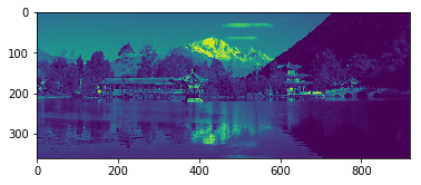
# 使用最大值代替每个像素点(最低维)
x = np.max(a, axis=2)
print(x)
plt.imshow(x)
[[0.827451   0.8156863  0.8156863  ... 0.02745098 0.02745098 0.03137255]
 [0.827451   0.8156863  0.8156863  ... 0.02745098 0.02745098 0.03137255]
 [0.8235294  0.8117647  0.8117647  ... 0.02745098 0.03137255 0.03137255]
 ...
 [0.56078434 0.56078434 0.5568628  ... 0.00392157 0.00392157 0.00392157]
 [0.5647059  0.56078434 0.5568628  ... 0.00392157 0.00392157 0.00392157]
 [0.5647059  0.56078434 0.5568628  ... 0.00392157 0.00392157 0.00392157]]


<matplotlib.image.AxesImage at 0x1596230a6a0>
# 使用最小值代替每个像素点(最低维)
x = np.min(a, axis=2)
print(x)
plt.imshow(x)
[[0.36862746 0.35686275 0.35686275 ... 0.00392157 0.00392157 0.00784314]
 [0.36862746 0.35686275 0.35686275 ... 0.00392157 0.00392157 0.00784314]
 [0.36862746 0.35686275 0.35686275 ... 0.00392157 0.00784314 0.00784314]
 ...
 [0.14117648 0.14117648 0.13725491 ... 0.00392157 0.00392157 0.00392157]
 [0.14509805 0.14117648 0.13725491 ... 0.00392157 0.00392157 0.00392157]
 [0.14509805 0.14117648 0.13725491 ... 0.00392157 0.00392157 0.00392157]]


<matplotlib.image.AxesImage at 0x159625fa8d0>
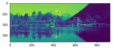
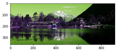
# 使用平均值代替每个像素点(最低维)
x = np.mean(a, axis=2)
print(x)
plt.imshow(x)
[[0.6039216  0.5921569  0.5921569  ... 0.0130719  0.0130719  0.01699346]
 [0.6039216  0.5921569  0.5921569  ... 0.0130719  0.0130719  0.01699346]
 [0.6026144  0.5908497  0.5908497  ... 0.0130719  0.01699346 0.01699346]
 ...
 [0.3503268  0.3503268  0.34640527 ... 0.00392157 0.00392157 0.00392157]
 [0.35424837 0.3503268  0.34640527 ... 0.00392157 0.00392157 0.00392157]
 [0.35424837 0.3503268  0.34640527 ... 0.00392157 0.00392157 0.00392157]]


<matplotlib.image.AxesImage at 0x1596279aa90>

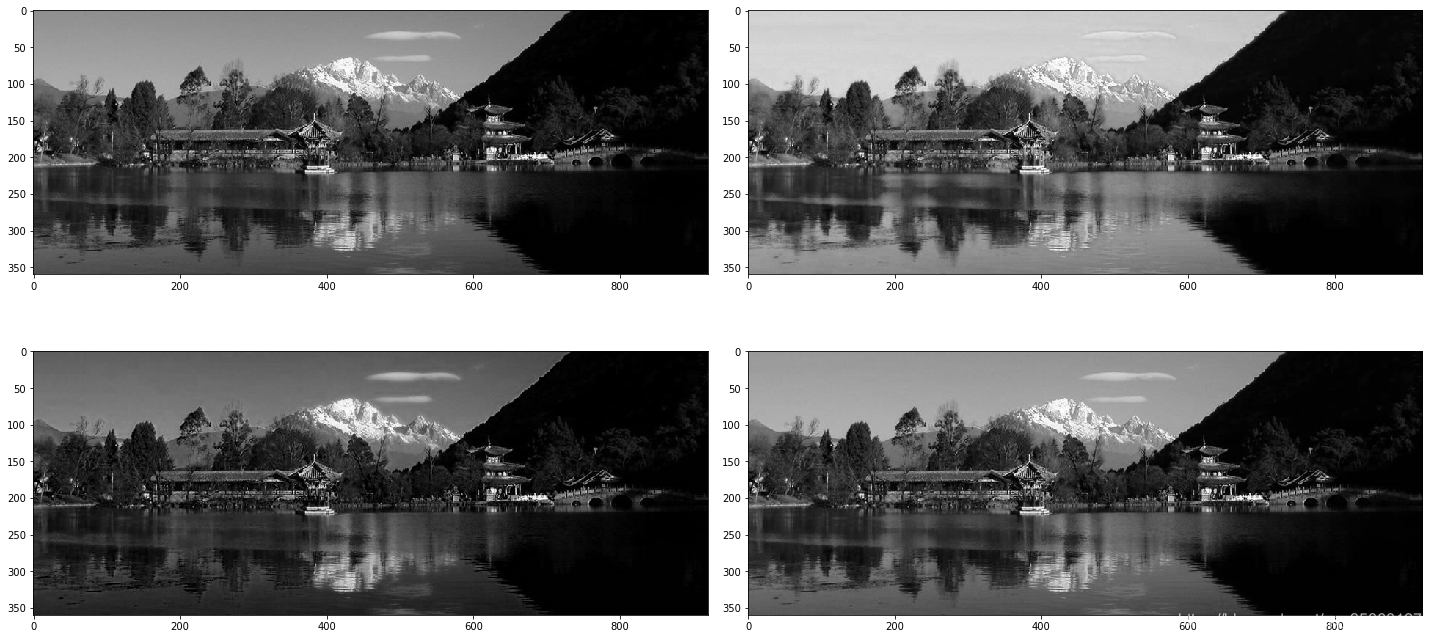
# 放在一起进行展示
fig, ax = plt.subplots(2, 2)
fig.set_size_inches(20, 10)
ax[0,0].imshow(np.dot(a, [0.299, 0.587, 0.114]), cmap="gray")
ax[0,1].imshow(np.max(a, axis=2), cmap="gray")
ax[1,0].imshow(np.min(a, axis=2), cmap="gray")
ax[1,1].imshow(np.mean(a, axis=2), cmap="gray")
plt.tight_layout()
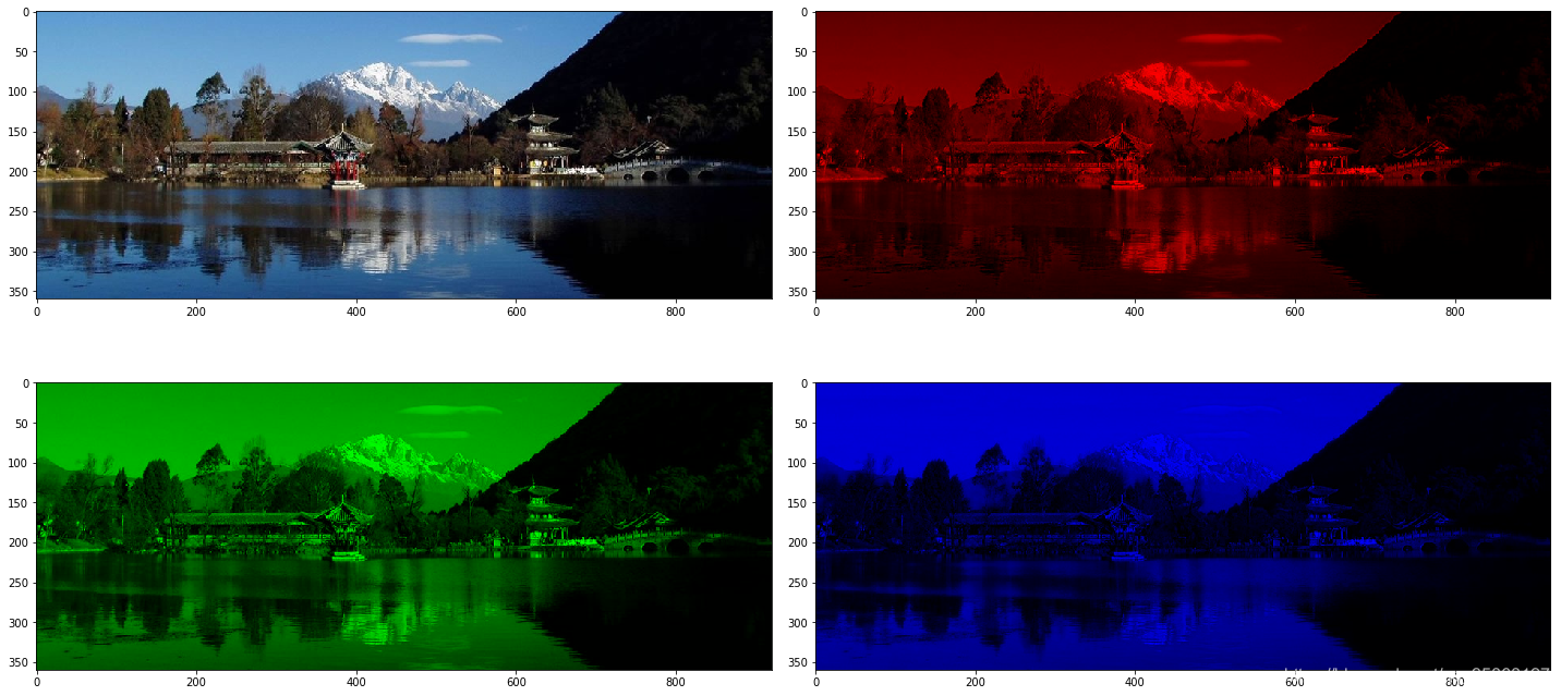
图像颜色通道
对于彩色图像,可以认为是由RGB三个通道构成的。每个最低维就是一个通道。分别提取R,G,B三个通道,并显示单通道的图像。
# 原图
plt.imshow(a)
<matplotlib.image.AxesImage at 0x15962fa3470>

x = a.copy()
# 拿出红色通道
x[:,:,1:3] = 0
print(x)
plt.imshow(x)
[[[0.36862746 0.         0.        ]
  [0.35686275 0.         0.        ]
  [0.35686275 0.         0.        ]
  ...
  [0.00784314 0.         0.        ]
  [0.00784314 0.         0.        ]
  [0.01176471 0.         0.        ]]

 [[0.36862746 0.         0.        ]
  [0.35686275 0.         0.        ]
  [0.35686275 0.         0.        ]
  ...
  [0.00784314 0.         0.        ]
  [0.00784314 0.         0.        ]
  [0.01176471 0.         0.        ]]

 [[0.36862746 0.         0.        ]
  [0.35686275 0.         0.        ]
  [0.35686275 0.         0.        ]
  ...
  [0.00784314 0.         0.        ]
  [0.01176471 0.         0.        ]
  [0.01176471 0.         0.        ]]

 ...

 [[0.14117648 0.         0.        ]
  [0.14117648 0.         0.        ]
  [0.13725491 0.         0.        ]
  ...
  [0.00392157 0.         0.        ]
  [0.00392157 0.         0.        ]
  [0.00392157 0.         0.        ]]

 [[0.14509805 0.         0.        ]
  [0.14117648 0.         0.        ]
  [0.13725491 0.         0.        ]
  ...
  [0.00392157 0.         0.        ]
  [0.00392157 0.         0.        ]
  [0.00392157 0.         0.        ]]

 [[0.14509805 0.         0.        ]
  [0.14117648 0.         0.        ]
  [0.13725491 0.         0.        ]
  ...
  [0.00392157 0.         0.        ]
  [0.00392157 0.         0.        ]
  [0.00392157 0.         0.        ]]]


<matplotlib.image.AxesImage at 0x15962ff39e8>

x = a.copy()
# 拿出绿色通道
# 数组索引
x[:,:,[0,2]] = 0     # x[:,:,::20] = 0   切片索引
print(x)
plt.imshow(x)
[[[0.         0.6156863  0.        ]
  [0.         0.6039216  0.        ]
  [0.         0.6039216  0.        ]
  ...
  [0.         0.00392157 0.        ]
  [0.         0.00392157 0.        ]
  [0.         0.00784314 0.        ]]

 [[0.         0.6156863  0.        ]
  [0.         0.6039216  0.        ]
  [0.         0.6039216  0.        ]
  ...
  [0.         0.00392157 0.        ]
  [0.         0.00392157 0.        ]
  [0.         0.00784314 0.        ]]

 [[0.         0.6156863  0.        ]
  [0.         0.6039216  0.        ]
  [0.         0.6039216  0.        ]
  ...
  [0.         0.00392157 0.        ]
  [0.         0.00784314 0.        ]
  [0.         0.00784314 0.        ]]

 ...

 [[0.         0.34901962 0.        ]
  [0.         0.34901962 0.        ]
  [0.         0.34509805 0.        ]
  ...
  [0.         0.00392157 0.        ]
  [0.         0.00392157 0.        ]
  [0.         0.00392157 0.        ]]

 [[0.         0.3529412  0.        ]
  [0.         0.34901962 0.        ]
  [0.         0.34509805 0.        ]
  ...
  [0.         0.00392157 0.        ]
  [0.         0.00392157 0.        ]
  [0.         0.00392157 0.        ]]

 [[0.         0.3529412  0.        ]
  [0.         0.34901962 0.        ]
  [0.         0.34509805 0.        ]
  ...
  [0.         0.00392157 0.        ]
  [0.         0.00392157 0.        ]
  [0.         0.00392157 0.        ]]]


<matplotlib.image.AxesImage at 0x159627f2c50>

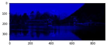
x = a.copy()
# 拿出蓝色通道
x[:,:,[0,1]] = 0
print(x)
plt.imshow(x)
[[[0.         0.         0.827451  ]
  [0.         0.         0.8156863 ]
  [0.         0.         0.8156863 ]
  ...
  [0.         0.         0.02745098]
  [0.         0.         0.02745098]
  [0.         0.         0.03137255]]

 [[0.         0.         0.827451  ]
  [0.         0.         0.8156863 ]
  [0.         0.         0.8156863 ]
  ...
  [0.         0.         0.02745098]
  [0.         0.         0.02745098]
  [0.         0.         0.03137255]]

 [[0.         0.         0.8235294 ]
  [0.         0.         0.8117647 ]
  [0.         0.         0.8117647 ]
  ...
  [0.         0.         0.02745098]
  [0.         0.         0.03137255]
  [0.         0.         0.03137255]]

 ...

 [[0.         0.         0.56078434]
  [0.         0.         0.56078434]
  [0.         0.         0.5568628 ]
  ...
  [0.         0.         0.00392157]
  [0.         0.         0.00392157]
  [0.         0.         0.00392157]]

 [[0.         0.         0.5647059 ]
  [0.         0.         0.56078434]
  [0.         0.         0.5568628 ]
  ...
  [0.         0.         0.00392157]
  [0.         0.         0.00392157]
  [0.         0.         0.00392157]]

 [[0.         0.         0.5647059 ]
  [0.         0.         0.56078434]
  [0.         0.         0.5568628 ]
  ...
  [0.         0.         0.00392157]
  [0.         0.         0.00392157]
  [0.         0.         0.00392157]]]


<matplotlib.image.AxesImage at 0x15962840e10>
red = a.copy()
green = a.copy()
blue = a.copy()
red[:, :, [1,2]] = 0
green[:, :, [0, 2]] = 0
blue[:, :, [0,1]] = 0
# 放在一起进行展示
fig, ax = plt.subplots(2, 2)
fig.set_size_inches(20, 10)
ax[0, 0].imshow(a)
ax[0, 1].imshow(red)
ax[1, 0].imshow(green)
ax[1, 1].imshow(blue)
plt.tight_layout()
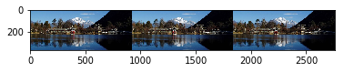
图像重复
- 将图像沿着水平方向重复三次。
- 将图像沿着垂直方向重复两次。
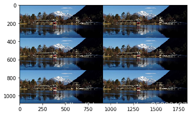
- 将图像沿着水平方向重复两次,垂直重复三次。
# 图像重复,只需要让数组的元素重复就可以。
# 数组的元素重复,可以使用数组拼接来实现。
# 将图像水平重复三次。
t = np.concatenate((a, a, a), axis=1)
plt.imshow(t)
<matplotlib.image.AxesImage at 0x15963a63898>
# 将图像垂直重复两次。
t = np.concatenate((a, a), axis=0)
plt.imshow(t)
<matplotlib.image.AxesImage at 0x15963ab3588>

# 将图像水平重复两次,垂直重复三次。
t = np.concatenate((a, a), axis=1)
t = np.concatenate((t, t, t), axis=0)
plt.imshow(t)
<matplotlib.image.AxesImage at 0x15963b0bd68>
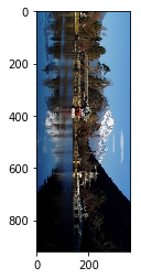
图像镜面对称
- 将图像水平镜面转换。
- 将图像垂直镜面转换。
# 原图
plt.imshow(a)
<matplotlib.image.AxesImage at 0x15963b6d400>

# 垂直镜面,水平对称。只需要将数组的行保持不变,列进行颠倒即可。
plt.imshow(a[:,::-1,:])
<matplotlib.image.AxesImage at 0x1596762c748>
# 水平镜面,垂直对称。只需要将数组的列保持不变,行进行颠倒即可。
plt.imshow(a[::-1])
<matplotlib.image.AxesImage at 0x15962f41b38>

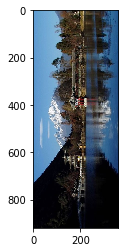
左右旋转
- 将图像向左旋转90 / 180度。
- 将图像向右旋转90 / 180度。
# 原图
plt.imshow(a)
<matplotlib.image.AxesImage at 0x1596308a278>

# 将图像向左旋转90度。可以将图像进行转置,然后进行垂直方向的颠倒。
# 注意,转置不能直接使用T属性,也不能直接使用无参的transpose。
# 1.将高与宽两个维度进行交换(转置)
t = a.swapaxes(0, 1)
plt.imshow(t)
<matplotlib.image.AxesImage at 0x1596766b2e8>
# 2.进行垂直方向的颠倒(对称)
t = t[::-1]
plt.imshow(t)
<matplotlib.image.AxesImage at 0x159629abac8>
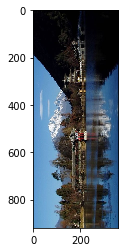
# 将图像向右旋转90度。可以将图像进行转置,然后进行水平方向的颠倒。
# 转置
t = a.swapaxes(0, 1)
# 进行水平方向的颠倒
t = t[:, ::-1]
plt.imshow(t)
<matplotlib.image.AxesImage at 0x159676994a8>
# 将图像旋转180度(左旋转与右旋转效果相同)。可以将图像分别进行一次水平颠倒与垂直颠倒。
# 1.进行垂直颠倒
t = a[::-1]
plt.imshow(t)
<matplotlib.image.AxesImage at 0x15962da4b00>
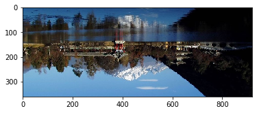
# 2.进行水平颠倒
t = t[:, ::-1]
plt.imshow(t)
<matplotlib.image.AxesImage at 0x15962df5f28>
[外链图片转存失败,源站可能有防盗链机制,建议将图片保存下来直接上传(img-9198tvWM-1577161964528)(output_40_1.png)]
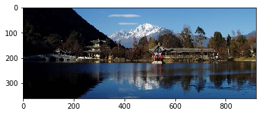
颜色转换
在图像中,用绿色值代替以前的红色值,用蓝色值代替以前的绿色值,用红色值代替以前的蓝色值。
t = a.copy()
plt.imshow(t[:, :, [1,2,0]])
<matplotlib.image.AxesImage at 0x15962e4f0f0>
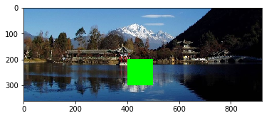
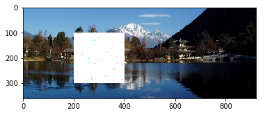
颜色遮挡 / 叠加
- 在指定的区域使用特定的纯色去遮挡图像。
- 在指定的区域使用随机生成的图像去遮挡图像。
- 使用小图像放在大图像上。
# 原图
plt.imshow(a)
<matplotlib.image.AxesImage at 0x15962e9d2e8>
t = a.copy()
t[200:300, 400:500] = [0, 255, 0]
plt.imshow(t)
Clipping input data to the valid range for imshow with RGB data ([0..1] for floats or [0..255] for integers).


<matplotlib.image.AxesImage at 0x159630ba668>
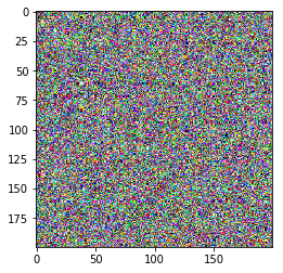
# 随机生成一个图像
k1 = np.random.randint(low=0, high=256, size=(200, 200, 3), dtype=np.uint8)
plt.imshow(k1)
<matplotlib.image.AxesImage at 0x1596310e860>
# 用随机生成的图片覆盖
t = a.copy()
t[100:300, 200:400] = k1
plt.imshow(t)
Clipping input data to the valid range for imshow with RGB data ([0..1] for floats or [0..255] for integers).


<matplotlib.image.AxesImage at 0x159631658d0>
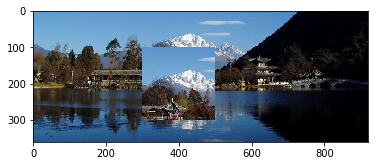
t = a.copy()
k2 = t[0:200, 300:500]
t[100:300, 300:500] = k2
plt.imshow(t)
<matplotlib.image.AxesImage at 0x159631b4d68>
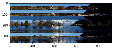
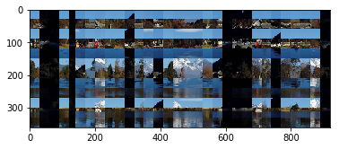
图像分块乱序
将图像分成若干块子图像(例如10 * 10),然后打乱各子图像顺序(拼图)。
# 原图
plt.imshow(a)
<matplotlib.image.AxesImage at 0x15963607978>

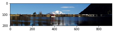
# 将图像的两部分进行组合。
t = a.copy()
t = np.concatenate((t[0:100], t[200:300]), axis=0)
plt.imshow(t)
<matplotlib.image.AxesImage at 0x15963655fd0>
# 分块操作。
# 1.切分图像,切成成若干块。【对数组数据进行切分】
# 2.洗牌,对数组数据打乱顺序
# 3.合并,将无序的数组合并在一起。

# 对数组数据进行切分。
print(a.shape)
t = a.copy()
high = a.shape[0]
li = np.split(t,range(30, high, 30),axis=0)
# 打乱数组元素的顺序。
np.random.shuffle(li)
# 合并乱序后的数组。
t = np.concatenate(li, axis=0)
plt.imshow(t)
(360, 920, 3)


<matplotlib.image.AxesImage at 0x159638c4e10>
# 在列的方向上再进行一次切分,组合。
width = a.shape[1]
li = np.split(t, range(30, width, 30), axis=1)
np.random.shuffle(li)
t = np.concatenate(li, axis=1)
plt.imshow(t)
<matplotlib.image.AxesImage at 0x159636b7da0>


 1718
1718


 被折叠的 条评论
为什么被折叠?
被折叠的 条评论
为什么被折叠?
 到【灌水乐园】发言


