PyTorch 入门学习（三）————搭建神经网络

神经网络

• 可以使用该torch.nn软件包构建神经网络
• 现在，您已经了解了autograd，这nn取决于 autograd定义模型并对其进行区分。一个nn.Module包含层，和输入值forward(input)，返回值output。
• 例子：以下对数字图像进行分类的网络
  
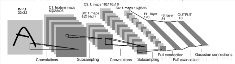
  这是一个简单的前馈网络。输入–隐藏层–输出层

神经网络的典型训练过程如下：

• 定义具有一些可学习参数（或权重）的神经网络
• 遍历输入数据集
• 通过网络处理输入
• 计算损失（输出离正确的距离还多远）
• 将梯度传播回网络参数
• 通常使用简单的更新规则来更新网络的权重：weight = weight - learning_rate * gradient

定义网络

1、 torch.nn.Conv2d （2d卷积核）

class torch.nn.Conv2d(in_channels, out_channels, kernel_size, stride=1, padding=0, dilation=1, groups=1, bias=True)

• in_channels(int) ：输入信号通道数
• out_channels(int) ： 卷积产生的通道
• kerner_size(int or tuple) ： 卷积核的尺寸
• stride(int or tuple, optional) ：卷积步长，默认为1
• padding(int or tuple, optional) ：输入的每一条边填充层数，默认为0
• dilation(int or tuple, optional) ： 卷积核元素之间的间距
• groups(int, optional) ：从输入通道到输出通道的阻塞连接数
• bias(bool, optional) ：如果bias=True，添加偏置

2、torch.nn.Linear

class torch.nn.Linear(in_features, out_features, bias=True)

对输入数据做线性变换：y = Ax + b

• in_features ：每个输入样本的大小
• out_features ： 每个输出样本的大小
• bias ： 若设置为False，这层不会学习偏置。默认值：True

3、torch.nn.functional.max_pool2d（最大2d池化层）

torch.nn.functional.max_pool2d(input, kernel_size, stride=None, padding=0, dilation=1, ceil_mode=False, return_indices=False)

4、torch.nn.functional.relu（非线性激活函数）

torch.nn.functional.relu(input, inplace=False)

import torch 
import torch.nn as nn
import torch.nn.functional as F


class Net(nn.Modile):  

    def __init__(self):
        super(Net, self).__init__()
        #1 input image channel, 6 output channels, 3x3 square convolution 设置第一个卷积核 C1 ，1个通道的输入，6个通道的输出，
        # kernel
        self.conv1 = nn.Conv2d(1, 6, 3)
        self.conv2 = nn.Conv2d(6, 16, 3)
        # an affine operation: y = Wx + b
        self.fc1 = nn.Linear(16 * 6 * 6, 120)  # 6*6 from image dimension
        self.fc2 = nn.Linear(120, 84)
        self.fc3 = nn.Linear(84, 10)
        
    def forward(self, x):
        # Max pooling over a (2, 2) window
        x = F.max_pool2d(F.relu(self.conv1(x)),(2, 2))
        #If the size is a square you can only specify a single number
        x = F.max_pool2d(F.relu(self.conv2(x)), 2)
        x = x.view(-1, self.num_flat_features(x)) #view函数将张量x变形成一维的向量形式，总特征数并不改变，为接下来的全连接作准备
        x = F.relu(self.fc1(x))
        x = F.relu(self.fc2(x))
        x = self.fc3(x)
        return x

    def num_flat_features(self, x):
        size = x.size()[1:]  # all dimensions except the batch dimension，这里为什么要使用[1:],是因为pytorch只接受批输入，也就是说一次性输入好几张图片，那么输入数据张量的维度自然上升到了4维。【1:】让我们把注意力放在后3维上面
        num_features = 1
        for s in size:
            num_features *= s
        return num_features

net = Net()
print(net)

输出：

Net(
  (conv1): Conv2d(1, 6, kernel_size=(3, 3), stride=(1, 1))
  (conv2): Conv2d(6, 16, kernel_size=(3, 3), stride=(1, 1))
  (fc1): Linear(in_features=576, out_features=120, bias=True)
  (fc2): Linear(in_features=120, out_features=84, bias=True)
  (fc3): Linear(in_features=84, out_features=10, bias=True)
)

只需要定义 forward 函数，backward 就可以使用 autograd 自动计算梯度，可以在 forward 函数中使用任何 Tensor 操作。

模型的可训练参数可以通过调用net.parameters()返回查看：

params = list(net.parameters())
print(len(params))
print(params[0].size())  # conv1's .weight

输出

10
torch.Size([6, 1, 3, 3])

让我们尝试一个32x32随机输入。注意：该网络的预期输入大小（LeNet）为32x32。要在MNIST数据集上使用此网络，请将图像从数据集中调整为32x32。

input = torch.randn(1, 1, 32, 32) # （样本数，通道数，高，宽）
out = net(input)
print(out)

输出

tensor([[-0.0330,  0.0880, -0.0362, -0.1725, -0.0252, -0.0873,  0.1195, -0.0958,
         -0.1148, -0.1005]], grad_fn=<AddmmBackward>)

用随机梯度将所有参数和反向传播器的梯度缓冲区归零：

net.zero_grad()
out.backward(torch.randn(1, 10))

• 注意：
• torch.nn仅支持小批量。整个torch.nn 程序包仅支持作为微型样本的输入，而不支持单个样本。
• 例如，nn.Conv2d将采用的4D张量 。nSamples x nChannels x Height x Width （样本数 x 通道数 x 高 x 宽）
• 如果您只有一个样本，则只需使用input.unsqueeze(0)即可添加伪造的批次尺寸。

至此，我们介绍了：

• 定义神经网络
• 处理输入以及调用反向传播

接下来：

• 计算损失
• 更新网络的权重

损失函数

损失函数采用一对（输出，目标）输入，并计算一个值，该值估计输出与目标的距离。

nn软件包下有几种不同的 损失函数。一个简单的损失是：nn.MSELoss计算输入和目标之间的均方误差。
例如：

output = net(input)
target = torch.randn(10)  # a dummy target, for example
target = target.view(1, -1)  # make it the same shape as output
criterion = nn.MSELoss()

loss = criterion(output, target)
print(loss)

输出

tensor(1.3691, grad_fn=<MseLossBackward>)

现在，如果loss使用.grad_fn属性的属性向后移动， 您将看到如下所示的计算图：

input -> conv2d -> relu -> maxpool2d -> conv2d -> relu -> maxpool2d
      -> view -> linear -> relu -> linear -> relu -> linear
      -> MSELoss
      -> loss

因此，当我们调用时loss.backward()，整个图与损失是微分的，并且图中的所有张量都requires_grad=True 将具有.grad随梯度累积的张量。
为了说明，让我们向后走几步：

print(loss.grad_fn)  # MSELoss
print(loss.grad_fn.next_functions[0][0])  # Linear
print(loss.grad_fn.next_functions[0][0].next_functions[0][0])  # ReLU

输出

<MseLossBackward object at 0x7f54dcac4128>
<AddmmBackward object at 0x7f54dcac4198>
<AccumulateGrad object at 0x7f54dcac4198>

反向传播

要实现反向传播，我们要做的是loss.backward()。不过，您需要清除现有的梯度，否则梯度将累积到现有的梯度中。现在我们将调用loss.backward()，并查看conv1的偏差梯度在反向传播前和反向传播之后的变化。

net.zero_grad()     # zeroes the gradient buffers of all parameters

print('conv1.bias.grad before backward')
print(net.conv1.bias.grad)

loss.backward()

print('conv1.bias.grad after backward')
print(net.conv1.bias.grad)

输出

conv1.bias.grad before backward
tensor([0., 0., 0., 0., 0., 0.])
conv1.bias.grad after backward
tensor([-0.0107, -0.0115,  0.0109,  0.0032,  0.0116,  0.0019])

更多模块和损失函数在这份完整的文档清单里
剩下要学习的是：

• 更新网络的权重

更新权重

实践中使用的最简单的更新规则是随机梯度下降（SGD）：

weight = weight - learning_rate * gradient

我们可以使用简单的python代码实现此目的：

learning_rate = 0.01
for f in net.parameters():
    f.data.sub_(f.grad.data * learning_rate)

但是，在使用神经网络时，您希望使用各种不同的更新规则，例如SGD，Nesterov-SGD，Adam，RMSProp等。为实现此目的，我们构建了一个小程序包：torch.optim实现所有这些方法。使用它非常简单：

import torch.optim as optim

# create your optimizer
optimizer = optim.SGD(net.parameters(), lr=0.01)

# in your training loop:
optimizer.zero_grad()   # zero the gradient buffers
output = net(input)
loss = criterion(output, target)
loss.backward()
optimizer.step()    # Does the update

完整代码