论文阅读笔记：（2018 ACCV）Cross Pixel Optical-Flow Similarity for Self-Supervised Learning

Cross Pixel Optical-Flow Similarity for Self-Supervised Learning

（2018 ACCV）

Aravindh Mahendran, James Thewlis, Andrea Vedaldi

Notes

Motivation

The authors propose a new self-supervised algorithm by using the optical flow that can be generated from videos in an unsupervised manner, and use stand alone from to train a model in a self-supervised setting. To avoid the difficulty of detecting specific details about the motion, such as direction and intensity, from a single frame, we learn to embed pixels into vectors that cluster together when the model believes that the corresponding pixels are likely to move together. This is obtained by encouraging the inner product of the learned pixel embeddings to correlate with the similarity between their corresponding optical flow vectors. But even objects that can move together may not do so all the time, such as objects stand still, and this was addresses by using a contrastive loss.

Method

Our goal is to learn the parameters of a neural network that maps a single image or frame to a field of pixel embeddings, one for each pixel. Our CNN is the per-pixel mapping producing D dimensional embeddings.

In order to learn this CNN, we require the similarity between pairs of embedding vectors to align with the similarity between the corresponding flow vectors. This is sufficient to capture the idea that things that move together should be grouped together. Given D-dimensional CNN embedding vectors   for pixels  and their corresponding flow vectors , we match the kernel matrices:

where  are kernels that measure the similarity of the CNN embeddings and flow vectors, respectively.

Kernels. In order to compare CNN embedding vectors and flow vectors, we choose the (scaled) cosine similarity kernel and the Gaussian/RBF kernel respectively. Using the shorthand notation  for readability, these are:

Note that these kernels, when restricted to the set of pixels Ω, are matrices of size .

Cross Pixel Optical-Flow Similarity Loss Function. The constraint in Eq. (1) requires kernels  and  to be similar. We experiment with three loss functions for this task - kernel target alignment, crossentropy, and cross-entropy reversed.

• Kernel Target Alignment (KTA): KTA is a conventional metric to measure the similarity between kernels. KTA for two kernel matrices , is given by

• Cross-Entropy (CE): Our second loss function treats pixels as classes and kernel values as logits of a distribution over pixels. The cross entropy of these two distributions measures the distance between them. We compute this loss in two steps. First, we renormalize each column  of each kernel matrix into a probability distribution  describes which image pixels  are likely to belong to the same segment as pixel , according to optical-flow.  describes the same but from the CNN embedding’s perspective. These distributions, arising from CNN and optical-flow kernels, are compared by using cross entropy, summed over columns:

• Cross-Entropy Reversed (CE-rev): Note that the particular ordering of distributions inside the cross entropy loss of Eq. 4 treats the distribution induced by the optical-flow kernel Sf as ground truth. The embedding is tasked with inducing a kernel such that its corresponding distribution  matches . As an ablation study we also experiment with the order of distributions reversed. In other words we use,

CNN Embedding Function. We design the embedding CNN as a hypercolumn head over a conventional CNN backbone such as AlexNet. The hypercolumn concatenates features from multiple depths so that our embedding can exploit high resolution details normally lost due to max- pooling layers. In more detail, the backbone is a CNN with activations at several layers: . We follow [31] and interpolate values for a given pixel location and concatenate them to form a hypercolumn . Specifically, sparse hypercolumns are built from the conv1, pool1, conv3, pool5 and fc7 AlexNet activations.

The hypercolumn is then projected non-linearly to the desired embedding  using a multi-layer perceptron (MLP). Embeddings are generated using a multi-layer perceptron (MLP) with a single hidden layer and are L2-normalized. The embeddings are D = 16 dimensional.

For training, we use the sparsification trick of [31] and restrict prediction and loss computation to a few randomly sampled pixels in every iteration. This reduces memory consumption and improves training convergence as pixels in the same image are highly correlated and redundant; via sampling we can reduce this correlation and train more efficiently.

Dataset

We extract 8 random frames from each video and compute optical-flow between those at times t and t+5 using the same (handcrafted) optical-flow method of [33,42].

Optical-flow vectors (fx,fy) are normalized logarithmically to lie between [−1, 1] during training, so that occasional large flows do not dominate learning. More precisely, the normalization is given by:

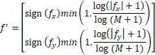
where M is a loose upper bound on the flow-magnitude set to 56.0 in our experiments.

Results