第四章：目标检测YoloV3（下）

多尺度检测

目前我们计算损失函数是在特征图P0的基础上进行的，它的步幅stride=32。特征图的尺寸比较小，像素点数目比较少，每个像素点的感受野很大，具有非常丰富的高层级语义信息，可能比较容易检测到较大的目标。为了能够检测到尺寸较小的那些目标，需要在尺寸较大的特征图上面建立预测输出。如果我们在C2或者C1这种层级的特征图上直接产生预测输出，可能面临新的问题，它们没有经过充分的特征提取，像素点包含的语义信息不够丰富，有可能难以提取到有效的特征模式。在目标检测中，解决这一问题的方式是，将高层级的特征图尺寸放大之后跟低层级的特征图进行融合，得到的新特征图既能包含丰富的语义信息，又具有较多的像素点，能够描述更加精细的结构。

具体的网络实现方式如 图19 所示：

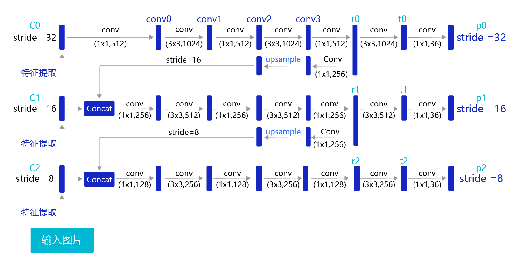
图19：生成多层级的输出特征图P0、P1、P2

YOLO-V3在每个区域的中心位置产生3个锚框，在3个层级的特征图上产生锚框的大小分别为P2 [(10×13),(16×30),(33×23)]，P1 [(30×61),(62×45),(59× 119)]，P0[(116 × 90), (156 × 198), (373 × 326]。越往后的特征图上用到的锚框尺寸也越大，能捕捉到大尺寸目标的信息；越往前的特征图上锚框尺寸越小，能捕捉到小尺寸目标的信息。

因为有多尺度的检测，所以需要对上面的代码进行较大的修改，而且实现过程也略显繁琐，所以推荐大家直接使用飞桨 fluid.layers.yolov3_loss API，关键参数说明如下：

paddle.fluid.layers.yolov3_loss(x, gt_box, gt_label, anchors, anchor_mask, class_num, ignore_thresh, downsample_ratio, gt_score=None, use_label_smooth=False, name=None)

• x: 输出特征图。
• gt_box: 真实框。
• gt_label: 真实框标签。
• ignore_thresh，预测框与真实框IoU阈值超过ignore_thresh时，不作为负样本，YOLO-V3模型里设置为0.7。
• downsample_ratio，特征图P0的下采样比例，使用Darknet53骨干网络时为32。
• gt_score，真实框的置信度，在使用了mixup技巧时用到。
• use_label_smooth，一种训练技巧，如不使用，设置为False。
• name，该层的名字，比如’yolov3_loss’，默认值为None，一般无需设置。

对于使用了多层级特征图产生预测框的方法，其具体实现代码如下：

# 定义上采样模块
class Upsample(fluid.dygraph.Layer):
    def __init__(self, scale=2):
        super(Upsample,self).__init__()
        self.scale = scale

    def forward(self, inputs):
        # get dynamic upsample output shape
        shape_nchw = fluid.layers.shape(inputs)
        shape_hw = fluid.layers.slice(shape_nchw, axes=[0], starts=[2], ends=[4])
        shape_hw.stop_gradient = True
        in_shape = fluid.layers.cast(shape_hw, dtype='int32')
        out_shape = in_shape * self.scale
        out_shape.stop_gradient = True

        # reisze by actual_shape
        out = fluid.layers.resize_nearest(
            input=inputs, scale=self.scale, actual_shape=out_shape)
        return out

# 定义YOLO-V3模型
class YOLOv3(fluid.dygraph.Layer):
    def __init__(self, num_classes=7, is_train=True):
        super(YOLOv3,self).__init__()

        self.is_train = is_train
        self.num_classes = num_classes
        # 提取图像特征的骨干代码
        self.block = DarkNet53_conv_body(
                                         is_test = not self.is_train)
        self.block_outputs = []
        self.yolo_blocks = []
        self.route_blocks_2 = []
        # 生成3个层级的特征图P0, P1, P2
        for i in range(3):
            # 添加从ci生成ri和ti的模块
            yolo_block = self.add_sublayer(
                "yolo_detecton_block_%d" % (i),
                YoloDetectionBlock(
                                   ch_in=512//(2**i)*2 if i==0 else 512//(2**i)*2 + 512//(2**i),
                                   ch_out = 512//(2**i),
                                   is_test = not self.is_train))
            self.yolo_blocks.append(yolo_block)

            num_filters = 3 * (self.num_classes + 5)

            # 添加从ti生成pi的模块，这是一个Conv2D操作，输出通道数为3 * (num_classes + 5)
            block_out = self.add_sublayer(
                "block_out_%d" % (i),
                Conv2D(num_channels=512//(2**i)*2,
                       num_filters=num_filters,
                       filter_size=1,
                       stride=1,
                       padding=0,
                       act=None,
                       param_attr=ParamAttr(
                           initializer=fluid.initializer.Normal(0., 0.02)),
                       bias_attr=ParamAttr(
                           initializer=fluid.initializer.Constant(0.0),
                           regularizer=L2Decay(0.))))
            self.block_outputs.append(block_out)
            if i < 2:
                # 对ri进行卷积
                route = self.add_sublayer("route2_%d"%i,
                                          ConvBNLayer(ch_in=512//(2**i),
                                                      ch_out=256//(2**i),
                                                      filter_size=1,
                                                      stride=1,
                                                      padding=0,
                                                      is_test=(not self.is_train)))
                self.route_blocks_2.append(route)
            # 将ri放大以便跟c_{i+1}保持同样的尺寸
            self.upsample = Upsample()

    def forward(self, inputs):
        outputs = []
        blocks = self.block(inputs)
        for i, block in enumerate(blocks):
            if i > 0:
                # 将r_{i-1}经过卷积和上采样之后得到特征图，与这一级的ci进行拼接
                block = fluid.layers.concat(input=[route, block], axis=1)
            # 从ci生成ti和ri
            route, tip = self.yolo_blocks[i](block)
            # 从ti生成pi
            block_out = self.block_outputs[i](tip)
            # 将pi放入列表
            outputs.append(block_out)

            if i < 2:
                # 对ri进行卷积调整通道数
                route = self.route_blocks_2[i](route)
                # 对ri进行放大，使其尺寸和c_{i+1}保持一致
                route = self.upsample(route)

        return outputs

    def get_loss(self, outputs, gtbox, gtlabel, gtscore=None,
                 anchors = [10, 13, 16, 30, 33, 23, 30, 61, 62, 45, 59, 119, 116, 90, 156, 198, 373, 326],
                 anchor_masks = [[6, 7, 8], [3, 4, 5], [0, 1, 2]],
                 ignore_thresh=0.7,
                 use_label_smooth=False):
        """
        使用fluid.layers.yolov3_loss，直接计算损失函数，过程更简洁，速度也更快
        """
        self.losses = []
        downsample = 32
        for i, out in enumerate(outputs): # 对三个层级分别求损失函数
            anchor_mask_i = anchor_masks[i]
            loss = fluid.layers.yolov3_loss(
                    x=out,  # out是P0, P1, P2中的一个
                    gt_box=gtbox,  # 真实框坐标
                    gt_label=gtlabel,  # 真实框类别
                    gt_score=gtscore,  # 真实框得分，使用mixup训练技巧时需要，不使用该技巧时直接设置为1，形状与gtlabel相同
                    anchors=anchors,   # 锚框尺寸，包含[w0, h0, w1, h1, ..., w8, h8]共9个锚框的尺寸
                    anchor_mask=anchor_mask_i, # 筛选锚框的mask，例如anchor_mask_i=[3, 4, 5]，将anchors中第3、4、5个锚框挑选出来给该层级使用
                    class_num=self.num_classes, # 分类类别数
                    ignore_thresh=ignore_thresh, # 当预测框与真实框IoU > ignore_thresh，标注objectness = -1
                    downsample_ratio=downsample, # 特征图相对于原图缩小的倍数，例如P0是32， P1是16，P2是8
                    use_label_smooth=False)      # 使用label_smooth训练技巧时会用到，这里没用此技巧，直接设置为False
            self.losses.append(fluid.layers.reduce_mean(loss))  #reduce_mean对每张图片求和
            downsample = downsample // 2 # 下一级特征图的缩放倍数会减半
        return sum(self.losses) # 对每个层级求和

开启端到端训练

训练过程如 图20 所示，输入图片经过特征提取得到三个层级的输出特征图P0(stride=32)、P1(stride=16)和P2(stride=8)，相应的分别使用不同大小的小方块区域去生成对应的锚框和预测框，并对这些锚框进行标注。

• P0层级特征图，对应着使用$32\times 32$大小的小方块，在每个区域中心生成大小分别为$[116,90]$, $[156,198]$, $[373,326]$的三种锚框。

• P1层级特征图，对应着使用$16\times 16$大小的小方块，在每个区域中心生成大小分别为$[30,61]$, $[62,45]$, $[59,119]$的三种锚框。

• P2层级特征图，对应着使用