从零开始数据科学与机器学习算法-线性回归-02

最新推荐文章于 2024-04-30 11:11:45 发布

gemoumou

最新推荐文章于 2024-04-30 11:11:45 发布

阅读量170

点赞数

分类专栏：数据科学与机器学习算法学习笔记文章标签：列表 python 数据分析机器学习算法

本文链接：https://blog.csdn.net/qq_37978800/article/details/114049271

版权

数据科学与机器学习算法学习笔记专栏收录该内容

14 篇文章 0 订阅

订阅专栏

简单线性回归

import numpy as np
import pandas as pd
import matplotlib.pyplot as plt
import seaborn as sns

问题1. The relationship between working experience and salary? 工作经验和工资之间的关系？

# 数据
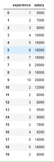
experience=[1,2,3,4,5,6,7,8,9,10,2,2,3,3,3,2,4,5,5,2]
salary    =[5000,7000,8000,10000,15000,18000,19000,20000,16000,30000,12000,6000,8000,5500,9000,7800,9200,14000,16000,8000]
# 数据合并
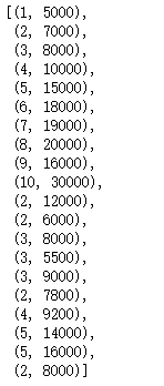
list_of_tuples=list(zip(experience,salary))
# 转换成dataframe类型
df=pd.DataFrame(list_of_tuples,columns=['experience','salary'])
df

在这里插入图片描述

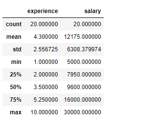
df.describe()#生成描述性统计

在这里插入图片描述

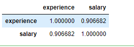
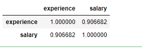
df.corr()

在这里插入图片描述

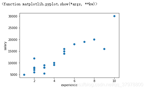
plt.scatter(df.experience,df.salary) # 绘制散点图
plt.xlabel('experience')
plt.ylabel('salary')
plt.show

在这里插入图片描述

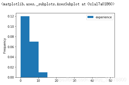
df.plot(kind="hist",y="experience",bins=10 ,range=(0,50),density= True)

在这里插入图片描述

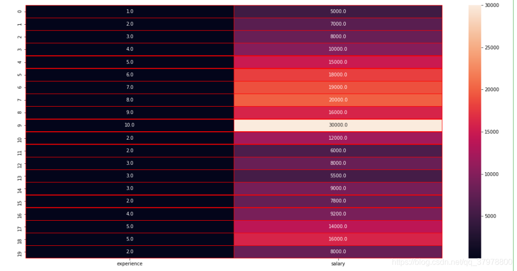
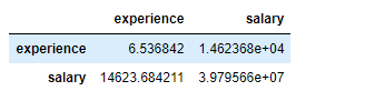
# 绘制热力图
f, ax =plt.subplots(figsize=(20,10))
sns.heatmap(df,annot=True,linewidths=0.5,linecolor="red",fmt=".1f",ax=ax)
plt.show()

在这里插入图片描述

#定义平均值计算函数
# First , Let's calculate the mean!
def calculate_mean(a_list_of_values): # 传入一组数据
    mean=sum(a_list_of_values)/float(len(a_list_of_values)) # 数据的总和除以数据的个数
    return mean # 返回平均值

# 计算方差函数
# Then , Let's calculate the variance!
def calculate_variance(a_list_of_values,mean):# 传入一组数据和平均值
    variance_sum=sum((x-mean)**2 for x in a_list_of_values)#  通过for循环遍历数据中的每个值  每个值减去数据的平方值的平方的总和
    variance=variance_sum/(len(a_list_of_values)-1) # 总和除以（数据个数-1）得出方差值
    return variance

# 测试
experience=[1,2,3,4,5,6,7,8,9,10,2,2,3,3,3,2,4,5,5,2]
salary    =[5000,7000,8000,10000,15000,18000,19000,20000,16000,30000,12000,6000,8000,5500,9000,7800,9200,14000,16000,8000]

mean_experience=calculate_mean(experience)
print(mean_experience)
variance_experience=calculate_variance(experience,mean_experience)
print(variance_experience)

在这里插入图片描述

mean_salary=calculate_mean(salary)
print(mean_salary)
variance_salary=calculate_variance(salary,mean_salary)
print(variance_salary)

在这里插入图片描述

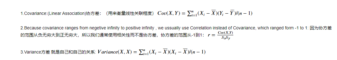
# And then we calculate the Covariance
#计算协方差
def calculate_covariance(a_list_of_Xs,the_mean_of_Xs,a_list_of_Ys,the_mean_of_Ys):# 传入x数据，x的平均值，y数据，y平均值
    cov_sum=0 # 首先定义结果为0通过下面循环+进去
    for i in range(len(a_list_of_Xs)):# 循环数据的长度
        cov_sum+=(a_list_of_Xs[i]-the_mean_of_Xs)*(a_list_of_Ys[i]-the_mean_of_Ys)#总和等于(x[i]-x_mean) 乘以 (y[i]-y_mean)
    the_covariance=cov_sum/(len(a_list_of_Xs)-1)#协方差等于 总和 除以（数据个数-1）
    return the_covariance

df.cov()# 调用pandas.DataFrame.cov协方差函数方法计算数据和我们自定义函数做验证

在这里插入图片描述

# 测试
covariance_of_experience_and_salary=calculate_covariance(experience,mean_experience,salary,mean_salary)
print(covariance_of_experience_and_salary)

在这里插入图片描述

# Let's calculate standard deviation!
# 计算标准差
def calculate_the_standard_deviation(a_list_values):
    the_mean_of_the_list_values=sum(a_list_values)/float(len(a_list_values))# 计算平均值
    variance=sum([(a_list_values[i]-the_mean_of_the_list_values)**2 for i in range(len(a_list_values)) ]) / float(len(a_list_values)-1)# sum（data[i]-mean）**2/(len(data)-1)
    return variance**0.5# 开方

# 测试标准差
a=[1,2,3,4,5,6,7,8,9,10]
calculate_the_standard_deviation(a) # 因为我们是计算样本的标准差 样本个数-1

在这里插入图片描述

import pandas as pd
b=np.array(a)
b.std() # 是计算整体的标准差
# 默认标准偏差类型在 numpy 的 .std() 和 pandas 的 .std() 函数之间是不同的。
# 默认情况下，numpy 计算的是总体标准偏差，ddof = 0。另一方面，pandas 计算的是样本标准偏差，ddof = 1。如果我们知道所有的分数，那么我们就有了总体——因此，要使用 pandas 进行归一化处理，我们需要将“ddof”设置为 0。

在这里插入图片描述

# Let's calculate the correlation!
# 计算相关性
def calculate_the_correlation(a_list_of_Xs,the_mean_of_Xs,a_list_of_Ys,the_mean_of_Ys):# 传入x数据，x的平均值，y数据，y平均值
    X_std=calculate_the_standard_deviation(a_list_of_Xs)# 使用标准差函数计算x数据标准差
    Y_std=calculate_the_standard_deviation(a_list_of_Ys) # 计算y数据标准差
    X_Y_Cov=calculate_covariance(a_list_of_Xs,the_mean_of_Xs,a_list_of_Ys,the_mean_of_Ys)# 使用协方差函数计算x，y的协方差
    
    Corr=(X_Y_Cov)/(X_std*Y_std) # 相关性等于 相关性除以（x标准差乘y标准差）
    return Corr

calculate_the_correlation(experience,mean_experience,salary,mean_salary)

在这里插入图片描述

df.corr()# 使用pandas—相关系数函数corr() 进行验证

在这里插入图片描述
Make Prediction: Use one variable to make prediction about another 预测：使用一个变量来预测另一个变量

dependent variable:Y 因变量y

independent variable:X 自变量x
• 回归分析(regression analysis)用来建立方程模拟两个或者多个变量之间如何关联 • 被预测的变量叫做：因变量(dependent variable), 输出(output) • 被用来进行预测的变量叫做：自变量(independent variable), 输入(input) • 一元线性回归包含一个自变量和一个因变量 • 以上两个变量的关系用一条直线来模拟 • 如果包含两个以上的自变量，则称作多元回归分析 (multiple regression)
在这里插入图片描述

# 计算系数
def calculate_the_coefficients(dataset):# 传入数据集
    x=[row[0] for row in dataset]# 循环数据集放入x和y中
    y=[row[1] for row in dataset]
    x_mean,y_mean=calculate_mean(x),calculate_mean(y) # 调用自定义平均函数算出x,y的平均值
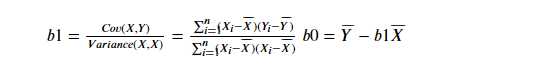
    b1=calculate_covariance(x,x_mean,y,y_mean)/calculate_variance(x,x_mean) # b1=（计算协方差（x数据，x平均值，y数据，y平均值） ）除以（方差（x数据，x平均值））
    b0=y_mean-b1*x_mean # b0 = y的平均值减去b1乘以x的平均值
    
    return [b0,b1]

# 数据
experience=[1,2,3,4,5,6,7,8,9,10,2,2,3,3,3,2,4,5,5,2]
salary    =[5000,7000,8000,10000,15000,18000,19000,20000,16000,30000,12000,6000,8000,5500,9000,7800,9200,14000,16000,8000]
# 数据合并
list_of_tuples=list(zip(experience,salary))
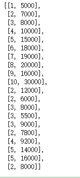
list_of_tuples

在这里插入图片描述

list_of_lists=[list(elem) for elem in list_of_tuples] # 将每个元素变成列表
list_of_lists

在这里插入图片描述

#测试系数
b0,b1=calculate_the_coefficients(list_of_lists) 
b0,b1

在这里插入图片描述
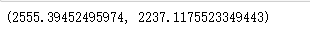
y=2555+2237X

# 简单线性回归函数
def simple_linear_regression(training_data,testing_data):# 传入参数
    predictions=[]# 定义个空列表存储预测结果
    b0,b1=calculate_the_coefficients(training_data)# 在相关系数函数中传入测试数据算出b0和b1
    for row in testing_data: # 循环测试数据
        y=b0+b1*row[0]# y等于b0+b1乘以测试数据的每个值
        predictions.append(y)
    return predictions

# 使用均方根误差来查看预测如何
from math import sqrt #  从math即数学库中导入用于开根运算的方法sqrt
def calculate_the_RMSE(predicted_data,actual_data):
    the_sum_of_error=0
    for i in range(len(actual_data)):
        prediction_error=predicted_data[i]-actual_data[i] # 循环遍历预测值和真实值相减的结果
        the_sum_of_error += (prediction_error**2) # 预测值和真实值相减的结果的平方
    RMSE=sqrt(the_sum_of_error/float(len(actual_data))) # 预测值和真实值相减的结果的平方除以数据个数的开根运算
    return RMSE

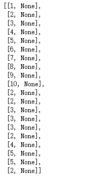
# 将数据分离只要工作年限最后在模型中预测出收入结果
data_to_be_put_into_the_model=[]
for row in list_of_lists:
    row_copy=list(row)
    row_copy[-1]=None
    data_to_be_put_into_the_model.append(row_copy)
data_to_be_put_into_the_model

在这里插入图片描述

# 利用模型预测收入结果
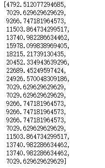
predictions=simple_linear_regression(list_of_lists,data_to_be_put_into_the_model) # 传入数据 传入分离出来的工作时间进行预测
predictions # 模型预测收入结果

在这里插入图片描述

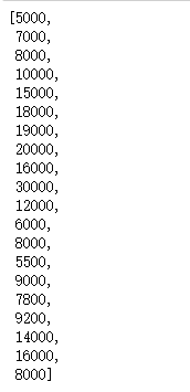
actual_data=[row[-1] for row in list_of_lists]# 提出真实收入做对比
actual_data

在这里插入图片描述

# 查看我们的模型有多好
def how_good_is_our_model(dataset,some_model_to_be_evaluated): # 真实值，模型评估的值
    test_data=[]
    for row in dataset:
        row_copy=list(row)
        row_copy[-1]=None
        test_data.append(row_copy)
    predict_data=some_model_to_be_evaluated(dataset,test_data)
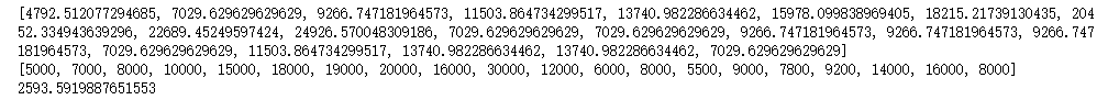
    print(predict_data)# 预测值
    actual_data=[row[-1] for row in dataset]
    print(actual_data) # 真实值
    RMSE=calculate_the_RMSE(predict_data,actual_data)
    return RMSE

result=how_good_is_our_model(list_of_lists,simple_linear_regression)
print(result) # 因原始数据很大 数据的量纲很大所以均方根误差结果也很大

在这里插入图片描述
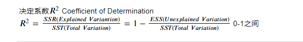
决定系数

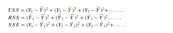
TSS = 真实值减平均值的平方
RSS = 预测值减去平均值的平方
SSE = 真实值减去预测值的平方

gemoumou

关注

0
点赞
踩
0

收藏

觉得还不错? 一键收藏
1
评论
从零开始数据科学与机器学习算法-线性回归-02

简单线性回归import numpy as npimport pandas as pdimport matplotlib.pyplot as pltimport seaborn as sns问题1. The relationship between working experience and salary? 工作经验和工资之间的关系？# 数据experience=[1,2,3,4,5,6,7,8,9,10,2,2,3,3,3,2,4,5,5,2]salary =[5000,7000
复制链接

扫一扫