Machine Learning(classifer)

Machine Learning

分类问题

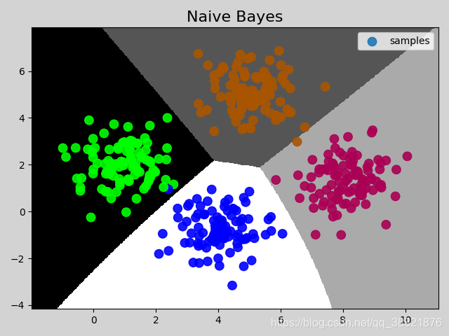
一.naive Bayes(朴素贝叶斯)

import numpy as np
import sklearn.naive_bayes as nb
import matplotlib.pyplot as mp

data = np.loadtxt(
    '../ml_data/multiple1.txt', delimiter=',')
x = data[:, :-1]
y = data[:, -1]
print(x.shape, y.shape)

# 拆分测试集训练集
import sklearn.model_selection as ms
train_x, test_x, train_y,  test_y = \
    ms.train_test_split(
        x, y, test_size=0.25, random_state=7)

# 训练模型
model = nb.GaussianNB()
model.fit(train_x, train_y)
pred_test_y = model.predict(test_x)
print(pred_test_y)
print(test_y)
print((pred_test_y == test_y).sum() / test_y.size)
# 在图像中绘制样本
mp.figure('Naive Bayes', facecolor='lightgray')
mp.title('Naive Bayes', fontsize=16)

# 绘制分类边界线
l, r = x[:, 0].min() - 1, x[:, 0].max() + 1
b, t = x[:, 1].min() - 1, x[:, 1].max() + 1
n = 500
grid_x, grid_y = np.meshgrid(np.linspace(l, r, n),
                             np.linspace(b, t, n))
mesh_x = np.column_stack((grid_x.ravel(),
                          grid_y.ravel()))
grid_z = model.predict(mesh_x)
grid_z = grid_z.reshape(grid_x.shape)
mp.pcolormesh(grid_x, grid_y, grid_z, cmap='gray')

mp.scatter(test_x[:, 0], test_x[:, 1], c=test_y,
           cmap='brg_r', label='samples', s=80, alpha=0.9)
mp.legend()
mp.show()

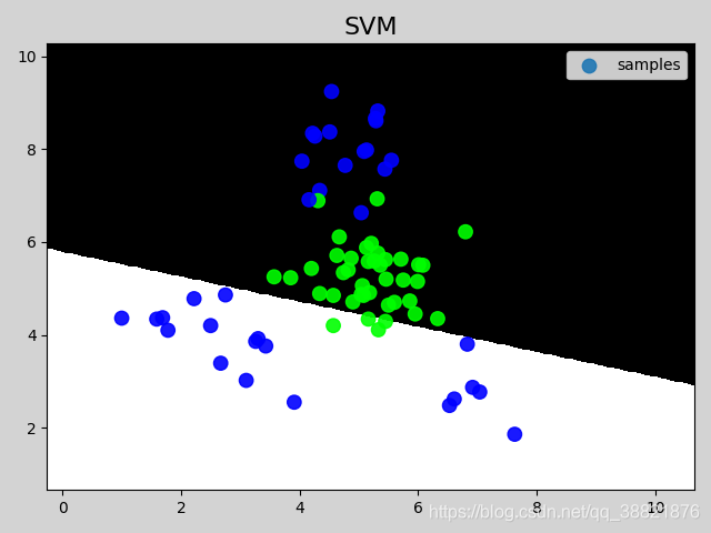
二.SVM(支持向量机)

linear 线性核函数

import numpy as np
import sklearn.naive_bayes as nb
import matplotlib.pyplot as mp
import sklearn.model_selection as ms
import sklearn.svm as svm

data = np.loadtxt(
    '../ml_data/multiple2.txt', delimiter=',')
x = data[:, :-1]
y = data[:, -1]
print(x.shape, y.shape)

# 拆分测试集训练集
train_x, test_x, train_y,  test_y = \
    ms.train_test_split(
        x, y, test_size=0.25, random_state=7)

# 训练模型
model = svm.SVC(kernel='linear')
model.fit(train_x, train_y)
pred_test_y = model.predict(test_x)

# 在图像中绘制样本
mp.figure('SVM', facecolor='lightgray')
mp.title('SVM', fontsize=16)

# 绘制分类边界线
l, r = x[:, 0].min() - 1, x[:, 0].max() + 1
b, t = x[:, 1].min() - 1, x[:, 1].max() + 1
n = 500
grid_x, grid_y = np.meshgrid(np.linspace(l, r, n),
                             np.linspace(b, t, n))
mesh_x = np.column_stack((grid_x.ravel(),
                          grid_y.ravel()))
grid_z = model.predict(mesh_x)
grid_z = grid_z.reshape(grid_x.shape)
mp.pcolormesh(grid_x, grid_y, grid_z, cmap='gray')

mp.scatter(test_x[:, 0], test_x[:, 1], c=test_y,
           cmap='brg_r', label='samples', s=80, alpha=0.9)
mp.legend()
mp.show()

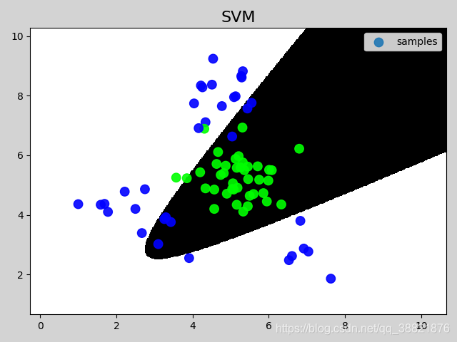
poly 线性核函数

import numpy as np
import sklearn.naive_bayes as nb
import matplotlib.pyplot as mp
import sklearn.model_selection as ms
import sklearn.svm as svm

data = np.loadtxt(
    '../ml_data/multiple2.txt', delimiter=',')
x = data[:, :-1]
y = data[:, -1]
print(x.shape, y.shape)

# 拆分测试集训练集
train_x, test_x, train_y,  test_y = \
    ms.train_test_split(
        x, y, test_size=0.25, random_state=7)

# 训练模型
model = svm.SVC(kernel='poly', degree=2)
model.fit(train_x, train_y)
pred_test_y = model.predict(test_x)
import sklearn.metrics as sm
print(sm.classification_report(test_y, pred_test_y))

# 在图像中绘制样本
mp.figure('SVM', facecolor='lightgray')
mp.title('SVM', fontsize=16)

# 绘制分类边界线
l, r = x[:, 0].min() - 1, x[:, 0].max() + 1
b, t = x[:, 1].min() - 1, x[:, 1].max() + 1
n = 500
grid_x, grid_y = np.meshgrid(np.linspace(l, r, n),
                             np.linspace(b, t, n))
mesh_x = np.column_stack((grid_x.ravel(),
                          grid_y.ravel()))
grid_z = model.predict(mesh_x)
grid_z = grid_z.reshape(grid_x.shape)
mp.pcolormesh(grid_x, grid_y, grid_z, cmap='gray')

mp.scatter(test_x[:, 0], test_x[:, 1], c=test_y,
           cmap='brg_r', label='samples', s=80, alpha=0.9)
mp.legend()
mp.show()

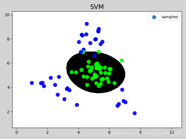
rbf 线函性核函数

import numpy as np
import sklearn.naive_bayes as nb
import matplotlib.pyplot as mp
import sklearn.model_selection as ms
import sklearn.svm as svm

data = np.loadtxt(
    '../ml_data/multiple2.txt', delimiter=',')
x = data[:, :-1]
y = data[:, -1]

print(x.shape, y.shape)

# 拆分测试集训练集
train_x, test_x, train_y,  test_y = \
    ms.train_test_split(
        x, y, test_size=0.25, random_state=7)

# 训练模型
model = svm.SVC(kernel='rbf', C=600, gamma=0.01)
model.fit(train_x, train_y)
pred_test_y = model.predict(test_x)
import sklearn.metrics as sm
print(sm.classification_report(test_y, pred_test_y))

# 在图像中绘制样本
mp.figure('SVM', facecolor='lightgray')
mp.title('SVM', fontsize=16)

# 绘制分类边界线
l, r = x[:, 0].min() - 1, x[:, 0].max() + 1
b, t = x[:, 1].min() - 1, x[:, 1].max() + 1
n = 500
grid_x, grid_y = np.meshgrid(np.linspace(l, r, n),
                             np.linspace(b, t, n))
mesh_x = np.column_stack((grid_x.ravel(),
                          grid_y.ravel()))
grid_z = model.predict(mesh_x)
grid_z = grid_z.reshape(grid_x.shape)
mp.pcolormesh(grid_x, grid_y, grid_z, cmap='gray')

mp.scatter(test_x[:, 0], test_x[:, 1], c=test_y,
           cmap='brg_r', label='samples', s=80, alpha=0.9)
mp.legend()
mp.show()

三.聚类

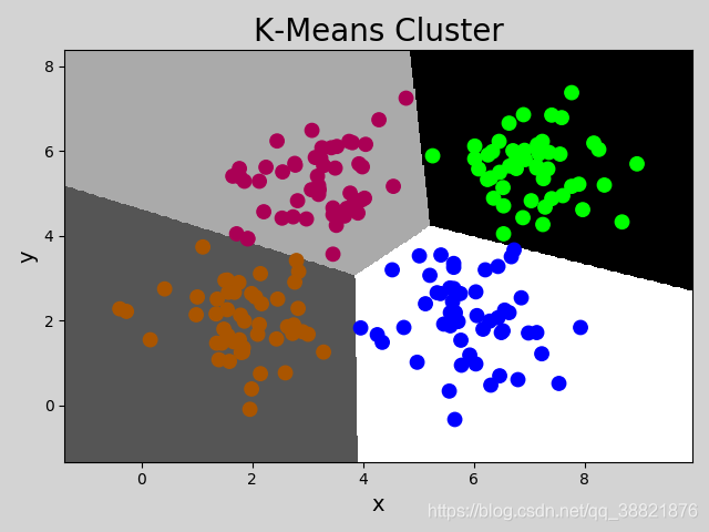
K-means算法

import numpy as np
import matplotlib.pyplot as mp
import sklearn.cluster as sc

x = np.loadtxt(
    '../ml_data/multiple3.txt', delimiter=',')
print(x.shape)
# 构建kmean模型
model = sc.KMeans(n_clusters=4)
model.fit(x)
labels = model.labels_
print(labels)

# 评估轮廓系数
import sklearn.metrics as sm
print(sm.silhouette_score(
    x, labels, sample_size=len(x), metric='euclidean'))

mp.figure('K-Means Cluster', facecolor='lightgray')
mp.title('K-Means Cluster', fontsize=20)
mp.xlabel('x', fontsize=14)
mp.ylabel('y', fontsize=14)
mp.tick_params(labelsize=10)


# 绘制分类边界线
l, r = x[:, 0].min() - 1, x[:, 0].max() + 1
b, t = x[:, 1].min() - 1, x[:, 1].max() + 1
n = 500
grid_x, grid_y = np.meshgrid(np.linspace(l, r, n),
                             np.linspace(b, t, n))
mesh_x = np.column_stack((grid_x.ravel(),
                          grid_y.ravel()))
grid_z = model.predict(mesh_x)
grid_z = grid_z.reshape(grid_x.shape)
mp.pcolormesh(grid_x, grid_y, grid_z, cmap='gray')


mp.scatter(x[:, 0], x[:, 1], c=labels, cmap='brg_r', s=80)
mp.show()

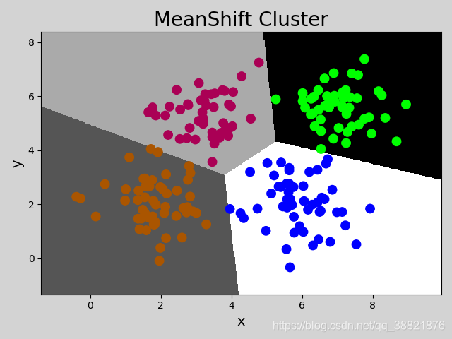
Meanshift Cluster(均值漂移算法)

import numpy as np
import matplotlib.pyplot as mp
import sklearn.cluster as sc

x = np.loadtxt(
    '../ml_data/multiple3.txt', delimiter=',')
print(x.shape)
# 构建meanshift模型
bw = sc.estimate_bandwidth(
    x, n_samples=len(x), quantile=0.1)
model = sc.MeanShift(bandwidth=bw, bin_seeding=True)
model.fit(x)
labels = model.labels_
print(labels)
print(model.cluster_centers_)
mp.figure('MeanShift Cluster', facecolor='lightgray')
mp.title('MeanShift Cluster', fontsize=20)
mp.xlabel('x', fontsize=14)
mp.ylabel('y', fontsize=14)
mp.tick_params(labelsize=10)


# 绘制分类边界线
l, r = x[:, 0].min() - 1, x[:, 0].max() + 1
b, t = x[:, 1].min() - 1, x[:, 1].max() + 1
n = 500
grid_x, grid_y = np.meshgrid(np.linspace(l, r, n),
                             np.linspace(b, t, n))
mesh_x = np.column_stack((grid_x.ravel(),
                          grid_y.ravel()))
grid_z = model.predict(mesh_x)
grid_z = grid_z.reshape(grid_x.shape)
mp.pcolormesh(grid_x, grid_y, grid_z, cmap='gray')


mp.scatter(x[:, 0], x[:, 1], c=labels, cmap='brg_r', s=80)
mp.show()

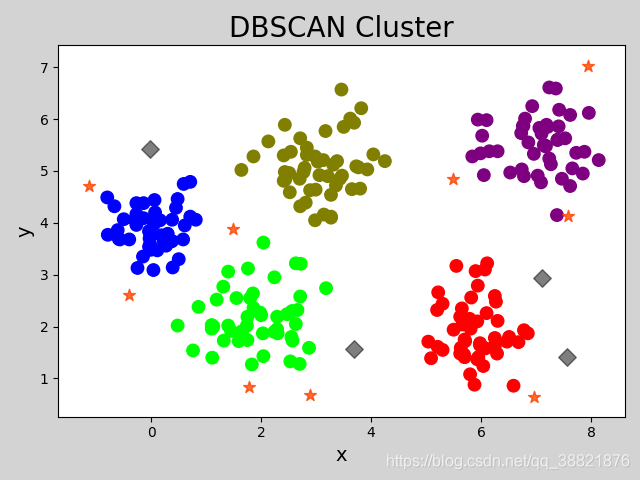
DBSCAN Cluster

import numpy as np
import matplotlib.pyplot as mp
import sklearn.cluster as sc
import sklearn.metrics as sm

x = np.loadtxt(
    '../ml_data/perf.txt', delimiter=',')

# 训练DBSCAN模型，借助轮廓系数优选最优半径
eps = np.linspace(0.2, 1.0, 9)
models, scores = [], []
for r in eps:
    model = sc.DBSCAN(eps=r, min_samples=5)
    model.fit(x)
    labels = model.labels_
    score = sm.silhouette_score(
        x, labels, sample_size=len(x),
        metric='euclidean')
    models.append(model)
    scores.append(score)

# 选出最优模型
best_ind = np.argmax(scores)
best_model = models[best_ind]
best_score = scores[best_ind]
best_eps = eps[best_ind]
print(best_eps, best_score)

mp.figure('DBSCAN Cluster', facecolor='lightgray')
mp.title('DBSCAN Cluster', fontsize=20)
mp.xlabel('x', fontsize=14)
mp.ylabel('y', fontsize=14)
mp.tick_params(labelsize=10)
# 使用最优模型绘制散点图像
labels = best_model.labels_
# 绘制所有核心样本的索引下标
core_inds = best_model.core_sample_indices_
mp.scatter(x[:, 0][core_inds], x[:, 1][core_inds],
           c=labels[core_inds], cmap='brg_r', s=80)

# 绘制所有孤立样本
offset_mask = labels == -1
mp.scatter(x[:, 0][offset_mask], x[:, 1][offset_mask],
           color='k', s=80, marker='D', alpha=0.5)

# 获取所有外周样本
mask = np.zeros(labels.size, dtype='bool')
mask[core_inds] = True
p_mask = ~(mask | offset_mask)
mp.scatter(x[:, 0][p_mask], x[:, 1][p_mask],
           color='orangered', s=80,
           marker='*', alpha=0.8)


mp.show()