


第2章 预备知识
2.1 数据操作
2.1.1 入门
导入的是torch而不是pytorch
import torch
一个数叫标量
一个轴叫向量
两个轴叫矩阵
arange
# 生成行向量
x = torch.arange(12)
x
tensor([ 0, 1, 2, 3, 4, 5, 6, 7, 8, 9, 10, 11])
shape
x.shape #访问张量的形状
torch.Size([12])
numel()
#访问张量中元素的个数
x.numel()
12
reshape()
x = x.reshape(3,4)
x
tensor([[ 0,  1,  2,  3],
        [ 4,  5,  6,  7],
        [ 8,  9, 10, 11]])
torch.zeros()
torch.zeros((2,3,4)) #2*3*4维度
tensor([[[0., 0., 0., 0.],
         [0., 0., 0., 0.],
         [0., 0., 0., 0.]],

        [[0., 0., 0., 0.],
         [0., 0., 0., 0.],
         [0., 0., 0., 0.]]])
torch.ones()
torch.ones((2,3,4))
tensor([[[1., 1., 1., 1.],
         [1., 1., 1., 1.],
         [1., 1., 1., 1.]],

        [[1., 1., 1., 1.],
         [1., 1., 1., 1.],
         [1., 1., 1., 1.]]])
torch.randn()
生成元素服从均值为0,标准差为1的正态分布
torch.randn(3,4)
tensor([[ 0.7507,  0.6205, -1.2569,  0.6519],
        [-2.0297,  0.7286, -0.0741, -0.7660],
        [-1.5470, -1.2288, -0.3673,  0.3899]])
torch.tensor()
numpy转换为Tensor
torch.tensor([[2,1,4,3],[1,2,3,4],[4,3,2,1]])
tensor([[2, 1, 4, 3],
        [1, 2, 3, 4],
        [4, 3, 2, 1]])
2.1.2 运算符
x = torch.tensor([1,2,4,8])
y = torch.tensor([2,2,2,2])
x+y, x-y, x*y, x/y, x**y
(tensor([ 3,  4,  6, 10]),
 tensor([-1,  0,  2,  6]),
 tensor([ 2,  4,  8, 16]),
 tensor([0.5000, 1.0000, 2.0000, 4.0000]),
 tensor([ 1,  4, 16, 64]))
x = torch.tensor([1.0,2,4,8])
y = torch.tensor([2,2,2,2])
x+y, x-y, x*y, x/y, x**y
(tensor([ 3.,  4.,  6., 10.]),
 tensor([-1.,  0.,  2.,  6.]),
 tensor([ 2.,  4.,  8., 16.]),
 tensor([0.5000, 1.0000, 2.0000, 4.0000]),
 tensor([ 1.,  4., 16., 64.]))
torch.exp()
torch.exp(x)
tensor([2.7183e+00, 7.3891e+00, 5.4598e+01, 2.9810e+03])
torch.cat()
X = torch.arange(12, dtype=torch.float32).reshape((3,4))
Y = torch.tensor([[2.0,1,4,3],[1,2,3,4],[4,3,2,1]])
torch.cat((X,Y), dim=0), torch.cat((X,Y), dim=1)  #dim=1按列
(tensor([[ 0.,  1.,  2.,  3.],
         [ 4.,  5.,  6.,  7.],
         [ 8.,  9., 10., 11.],
         [ 2.,  1.,  4.,  3.],
         [ 1.,  2.,  3.,  4.],
         [ 4.,  3.,  2.,  1.]]),
 tensor([[ 0.,  1.,  2.,  3.,  2.,  1.,  4.,  3.],
         [ 4.,  5.,  6.,  7.,  1.,  2.,  3.,  4.],
         [ 8.,  9., 10., 11.,  4.,  3.,  2.,  1.]]))
X == Y
tensor([[False,  True, False,  True],
        [False, False, False, False],
        [False, False, False, False]])
X.sum()
X.sum()
tensor(66.)
a = torch.arange(3).reshape((3,1))
b = torch.arange(2).reshape((1,2))
a,b
(tensor([[0],
         [1],
         [2]]),
 tensor([[0, 1]]))
2.1.3 广播机制
#a为列向量,b为行向量
a+b  #广播机制
tensor([[0, 1],
        [1, 2],
        [2, 3]])
2.1.4 索引和切片
print(X)
print(X[-1])  #访问最后一行
print(X[1:3]) #访问索引为1,2的行
tensor([[ 0.,  1.,  2.,  3.],
        [ 4.,  5.,  6.,  7.],
        [ 8.,  9., 10., 11.]])
tensor([ 8.,  9., 10., 11.])
tensor([[ 4.,  5.,  6.,  7.],
        [ 8.,  9., 10., 11.]])
X[1,2] = 9  # 赋值
X
tensor([[ 0.,  1.,  2.,  3.],
        [ 4.,  5.,  9.,  7.],
        [ 8.,  9., 10., 11.]])
X[0:2, :] = 12
X
tensor([[12., 12., 12., 12.],
        [12., 12., 12., 12.],
        [ 8.,  9., 10., 11.]])
2.1.5 节省内存
before = id(Y)
Y = Y+X
id(Y) == before  #运行一些操作可能导致为新结果分配内存
False
zeros_like(Y)即形状与Y一致的全零矩阵
Z = torch.zeros_like(Y)
print(id(Z))
Z[:] = X+Y   #原地操作
print(id(Z))
2435091263384
2435091263384
before = id(X)
X += Y #不同于赋值
id(X) == before
True
得出结论:X[:]=X+Y或X+=Y可以减少操作的内存开销
2.1.6 array和Tensor类型相互转换
A = X.numpy()
B = torch.tensor(A)
type(A), type(B)
(numpy.ndarray, torch.Tensor)
2.2 数据预处理
2.2.1. 读取数据集
先生成一个数据集:其中每行描述了房间数量(“NumRooms”)、巷子类型(“Alley”)和房屋价格(“Price”)。
import os

os.makedirs(os.path.join('.','data'), exist_ok=True)
data_file = os.path.join('.', 'data', 'house_tiny.csv')
with open(data_file, 'w') as f:
    f.write('NumRooms,Alley,Price\n')  # 列名
    f.write('NA,Pave,127500\n')  # 每行表示一个数据样本
    f.write('2,NA,106000\n')
    f.write('4,NA,178100\n')
    f.write('NA,NA,140000\n')
再读取数据集
# 如果没有安装pandas,只需取消对以下行的注释来安装pandas
# !pip install pandas
import pandas as pd

data = pd.read_csv(data_file)
print(data)
   NumRooms Alley   Price
0       NaN  Pave  127500
1       2.0   NaN  106000
2       4.0   NaN  178100
3       NaN   NaN  140000
2.2.2. 处理缺失值
#划分输入输出
inputs, outputs = data.iloc[:, 0:2], data.iloc[:, 2]

#对输出进行预处理
inputs = inputs.fillna(inputs.mean())
print(inputs)
   NumRooms Alley
0       3.0  Pave
1       2.0   NaN
2       4.0   NaN
3       3.0   NaN
对于inputs中的类别值或离散值,我们将“NaN”视为一个类别。
inputs = pd.get_dummies(inputs, dummy_na=True)
print(inputs)
   NumRooms  Alley_Pave  Alley_nan
0       3.0           1          0
1       2.0           0          1
2       4.0           0          1
3       3.0           0          1
可见输入为3*4矩阵
上面数据都是array类型,用pandas和numpy处理;下面转换成Tensor
2.2.3. 转换为张量格式
X:34
y:41
import torch

X, y = torch.tensor(inputs.values), torch.tensor(outputs.values)
X, y
(tensor([[3., 1., 0.],
         [2., 0., 1.],
         [4., 0., 1.],
         [3., 0., 1.]], dtype=torch.float64),
 tensor([127500, 106000, 178100, 140000]))
2.3 线性代数
2.3.1 标量
标量由只有一个元素的张量表示
import torch

x = torch.tensor(3.0)
y = torch.tensor(2.0)

x + y, x * y, x / y, x**y
(tensor(5.), tensor(6.), tensor(1.5000), tensor(9.))
2.3.2 向量
向量可以视为由标量值组成的列表
x = torch.arange(4)
x
tensor([0, 1, 2, 3])
大量文献认为列向量是向量的默认方向,这里也是默认此
x[3]
tensor(3)
2.3.2.1. 长度、维度和形状
向量只是一个数组,数组有长度,没向量也如此
len(x)
4
当用张量表示一个向量(只有一个轴)时,我们也可以通过.shape属性访问向量的长度。
x.shape
torch.Size([4])
2.3.3 矩阵
A = torch.arange(20).reshape(5, 4)
A
tensor([[ 0,  1,  2,  3],
        [ 4,  5,  6,  7],
        [ 8,  9, 10, 11],
        [12, 13, 14, 15],
        [16, 17, 18, 19]])
转置
A.T
tensor([[ 0,  4,  8, 12, 16],
        [ 1,  5,  9, 13, 17],
        [ 2,  6, 10, 14, 18],
        [ 3,  7, 11, 15, 19]])
对称矩阵
B = torch.tensor([[1, 2, 3], [2, 0, 4], [3, 4, 5]])
B
tensor([[1, 2, 3],
        [2, 0, 4],
        [3, 4, 5]])
B == B.T
tensor([[True, True, True],
        [True, True, True],
        [True, True, True]])
2.3.4 张量
向量是标量的推广,矩阵是向量的推广
向量是一阶张量,矩阵是二阶张量
X = torch.arange(24).reshape(2, 3, 4)
X
tensor([[[ 0,  1,  2,  3],
         [ 4,  5,  6,  7],
         [ 8,  9, 10, 11]],

        [[12, 13, 14, 15],
         [16, 17, 18, 19],
         [20, 21, 22, 23]]])
2.3.5 张量算法的基本性质
A = torch.arange(20, dtype=torch.float32).reshape(5, 4)
B = A.clone()  # 通过分配新内存,将A的一个副本分配给B
A, A + B
(tensor([[ 0.,  1.,  2.,  3.],
         [ 4.,  5.,  6.,  7.],
         [ 8.,  9., 10., 11.],
         [12., 13., 14., 15.],
         [16., 17., 18., 19.]]),
 tensor([[ 0.,  2.,  4.,  6.],
         [ 8., 10., 12., 14.],
         [16., 18., 20., 22.],
         [24., 26., 28., 30.],
         [32., 34., 36., 38.]]))
A * B #点乘 对应元素相乘
tensor([[  0.,   1.,   4.,   9.],
        [ 16.,  25.,  36.,  49.],
        [ 64.,  81., 100., 121.],
        [144., 169., 196., 225.],
        [256., 289., 324., 361.]])
a = 2
X = torch.arange(24).reshape(2, 3, 4)
a + X, (a * X).shape
(tensor([[[ 2,  3,  4,  5],
          [ 6,  7,  8,  9],
          [10, 11, 12, 13]],

         [[14, 15, 16, 17],
          [18, 19, 20, 21],
          [22, 23, 24, 25]]]),
 torch.Size([2, 3, 4]))
2.3.6. 降维
一阶张量求和
x = torch.arange(4, dtype=torch.float32)
x, x.sum()
(tensor([0., 1., 2., 3.]), tensor(6.))
二阶张量求和
A
tensor([[ 0.,  1.,  2.,  3.],
        [ 4.,  5.,  6.,  7.],
        [ 8.,  9., 10., 11.],
        [12., 13., 14., 15.],
        [16., 17., 18., 19.]])
A.shape, A.sum()
(torch.Size([5, 4]), tensor(190.))
对每一列求和
A_sum_axis0 = A.sum(axis=0)
A_sum_axis0, A_sum_axis0.shape
(tensor([40., 45., 50., 55.]), torch.Size([4]))
对每一行求和
A_sum_axis1 = A.sum(axis=1)
A_sum_axis1, A_sum_axis1.shape
(tensor([ 6., 22., 38., 54., 70.]), torch.Size([5]))
对整个矩阵元素求和
A.sum(axis=[0, 1]) # SameasA.sum()
tensor(190.)
A.mean()
整个矩阵求均值
A.mean(), A.sum() / A.numel()
(tensor(9.5000), tensor(9.5000))
对每一列求均值
A.mean(axis=0), A.sum(axis=0) / A.shape[0]
(tensor([ 8., 9., 10., 11.]), tensor([ 8., 9., 10., 11.]))
2.3.6.1. 非降维求和
指定参数keepdims=True
sum_A = A.sum(axis=1, keepdims=True)
sum_A
tensor([[ 6.],
        [22.],
        [38.],
        [54.],
        [70.]])
由于sum_A在对每行进行求和后仍保持两个轴,我们可以通过广播将A除以sum_A。
A / sum_A
tensor([[0.0000, 0.1667, 0.3333, 0.5000],
        [0.1818, 0.2273, 0.2727, 0.3182],
        [0.2105, 0.2368, 0.2632, 0.2895],
        [0.2222, 0.2407, 0.2593, 0.2778],
        [0.2286, 0.2429, 0.2571, 0.2714]])
如果我们想沿某个轴计算A元素的累积总和, 比如axis=0(按行计算),我们可以调用cumsum函数。 此函数不会沿任何轴降低输入张量的维度。
A.cumsum(axis=0)
tensor([[ 0.,  1.,  2.,  3.],
        [ 4.,  6.,  8., 10.],
        [12., 15., 18., 21.],
        [24., 28., 32., 36.],
        [40., 45., 50., 55.]])
可以看出:第二行+=第一行
2.3.7. 点积(Dot Product)
对应点相乘再求和
y = torch.ones(4, dtype = torch.float32)
x, y, torch.dot(x, y)
(tensor([0., 1., 2., 3.]), tensor([1., 1., 1., 1.]), tensor(6.))
2.3.8. 矩阵-向量积
A.shape, x.shape, torch.mv(A, x)
(torch.Size([5, 4]), torch.Size([4]), tensor([ 14., 38., 62., 86., 110.]))
(5,4)(4,1)==(5,1)
2.3.9. 矩阵-矩阵乘法
B = torch.ones(4, 3)
torch.mm(A, B)
tensor([[ 6.,  6.,  6.],
        [22., 22., 22.],
        [38., 38., 38.],
        [54., 54., 54.],
        [70., 70., 70.]])
(5,4)(4,3)==(5,3)
2.3.10. 范数
L2 范数是向量元素平方和的平方根
# 计算向量的L2范数
u = torch.tensor([3.0, -4.0])
torch.norm(u)
tensor(5.)
L1 范数,它表示为向量元素的绝对值之和:
torch.abs(u).sum()
tensor(7.)
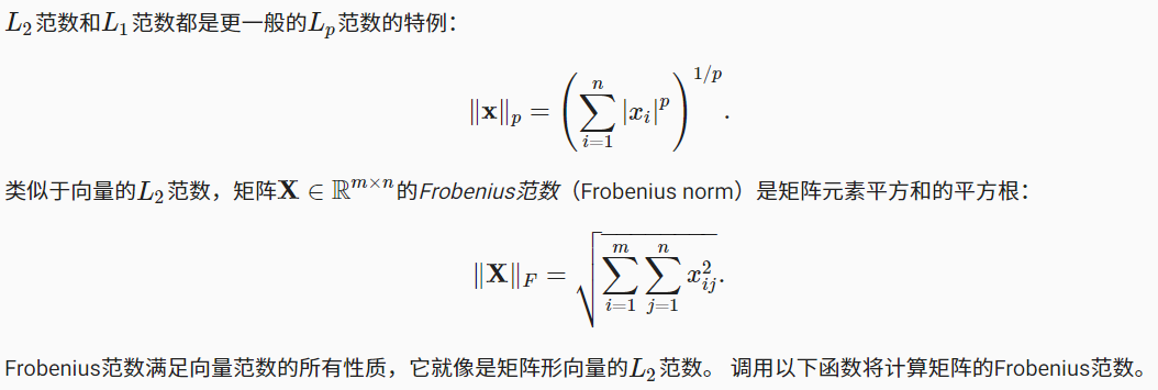
矩阵的L2范数称为F范数
torch.norm(torch.ones((4, 9)))
tensor(6.)
2.3.10.1. 范数和目标
在深度学习中,我们经常试图解决优化问题: 最大化分配给观测数据的概率; 最小化预测和真实观测之间的距离。
范数用来防止过拟合
2.4. 微积分
2.4.1. 导数和微分
%matplotlib inline
import numpy as np
from IPython import display
from d2l import torch as d2l


def f(x):
    return 3 * x ** 2 - 4 * x
def numerical_lim(f, x, h):
    return (f(x + h) - f(x)) / h

h = 0.1
for i in range(5):
    print(f'h={h:.5f}, numerical limit={numerical_lim(f, 1, h):.5f}')
    h *= 0.1
h=0.10000, numerical limit=2.30000
h=0.01000, numerical limit=2.03000
h=0.00100, numerical limit=2.00300
h=0.00010, numerical limit=2.00030
h=0.00001, numerical limit=2.00003
为了对导数的这种解释进行可视化,我们将使用matplotlib, 这是一个Python中流行的绘图库。 要配置matplotlib生成图形的属性,我们需要定义几个函数。 在下面,use_svg_display函数指定matplotlib软件包输出svg图表以获得更清晰的图像。
注意,注释#@save是一个特殊的标记,会将对应的函数、类或语句保存在d2l包中
def use_svg_display():  #@save
    """使用svg格式在Jupyter中显示绘图"""
    display.set_matplotlib_formats('svg')
我们定义set_figsize函数来设置图表大小。 注意,这里我们直接使用d2l.plt,因为导入语句 from matplotlib import pyplot as plt已标记为保存到d2l包中。
def set_figsize(figsize=(3.5, 2.5)):  #@save
    """设置matplotlib的图表大小"""
    use_svg_display()
    d2l.plt.rcParams['figure.figsize'] = figsize
下面的set_axes函数用于设置由matplotlib生成图表的轴的属性。
#@save
def set_axes(axes, xlabel, ylabel, xlim, ylim, xscale, yscale, legend):
    """设置matplotlib的轴"""
    axes.set_xlabel(xlabel)
    axes.set_ylabel(ylabel)
    axes.set_xscale(xscale)
    axes.set_yscale(yscale)
    axes.set_xlim(xlim)
    axes.set_ylim(ylim)
    if legend:
        axes.legend(legend)
    axes.grid()
通过这三个用于图形配置的函数,我们定义了plot函数来简洁地绘制多条曲线, 因为我们需要在整个书中可视化许多曲线。
#@save
def plot(X, Y=None, xlabel=None, ylabel=None, legend=None, xlim=None,
         ylim=None, xscale='linear', yscale='linear',
         fmts=('-', 'm--', 'g-.', 'r:'), figsize=(3.5, 2.5), axes=None):
    """绘制数据点"""
    if legend is None:
        legend = []

    set_figsize(figsize)
    axes = axes if axes else d2l.plt.gca()

    # 如果X有一个轴,输出True
    def has_one_axis(X):
        return (hasattr(X, "ndim") and X.ndim == 1 or isinstance(X, list)
                and not hasattr(X[0], "__len__"))

    if has_one_axis(X):
        X = [X]
    if Y is None:
        X, Y = [[]] * len(X), X
    elif has_one_axis(Y):
        Y = [Y]
    if len(X) != len(Y):
        X = X * len(Y)
    axes.cla()
    for x, y, fmt in zip(X, Y, fmts):
        if len(x):
            axes.plot(x, y, fmt)
        else:
            axes.plot(y, fmt)
    set_axes(axes, xlabel, ylabel, xlim, ylim, xscale, yscale, legend)
现在我们可以绘制函数 u=f(x) 及其在 x=1 处的切线 y=2x−3 , 其中系数 2 是切线的斜率。
x = np.arange(0, 3, 0.1)
plot(x, [f(x), 2 * x - 3], 'x', 'f(x)', legend=['f(x)', 'Tangent line (x=1)'])
[外链图片转存失败,源站可能有防盗链机制,建议将图片保存下来直接上传(img-bkNd6643-1640697045692)(https://gitee.com/zdbya/picgo_image/raw/master/SSL_img/202112282107422.svg+xml)]
2.4.6. 练习
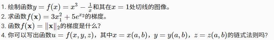
plot(x, [x**3-1/x, 4*x-4], 'x', 'f(x)', legend=['f(x)', 'Tangent line(x=1)'])
C:\programming_software\anaconda3\envs\learning_pytorch\lib\site-packages\ipykernel_launcher.py:1: RuntimeWarning: divide by zero encountered in true_divide
  """Entry point for launching an IPython kernel.
[外链图片转存失败,源站可能有防盗链机制,建议将图片保存下来直接上传(img-dEfxgucA-1640697045694)(https://gitee.com/zdbya/picgo_image/raw/master/SSL_img/202112281245547.svg)]
2.5 自动微分
深度学习框架通过自动计算导数,即自动微分(automatic differentiation)来加快求导。
实际中,根据我们设计的模型,系统会构建一个计算图(computational graph), 来跟踪计算是哪些数据通过哪些操作组合起来产生输出。
自动微分使系统能够随后反向传播梯度。 这里,反向传播(backpropagate)意味着跟踪整个计算图,填充关于每个参数的偏导数。
2.5.1 一个简单的例子
import torch

x = torch.arange(4.0)
x
tensor([0., 1., 2., 3.])
梯度存储在gird里面
x.requires_grad_(True)  # 等价于x=torch.arange(4.0,requires_grad=True)
x.grad  # 默认值是None
y=2x^2
y = 2 * torch.dot(x, x)
y
tensor(28., grad_fn=<MulBackward0>)
反向传播
y.backward()
x.grad
tensor([ 0., 4., 8., 12.])
x.grad == 4 * x
tensor([True, True, True, True])
现在让我们计算x的另一个函数。
# 在默认情况下,PyTorch会累积梯度,我们需要清除之前的值
x.grad.zero_()   #梯度清零
y = x.sum()
print(x)
print(y)

y.backward()
x.grad
tensor([0., 1., 2., 3.], requires_grad=True)
tensor(6., grad_fn=<SumBackward0>)


tensor([1., 1., 1., 1.])
2.5.2 非标量变量的方向传播
注意:深度学习一般是对变量求导,因为loss是标量
# 对非标量调用backward需要传入一个gradient参数,该参数指定微分函数关于self的梯度。
# 在我们的例子中,我们只想求偏导数的和,所以传递一个1的梯度是合适的
x.grad.zero_()
y = x * x
# 等价于y.backward(torch.ones(len(x)))
y.sum().backward()
x.grad
tensor([0., 2., 4., 6.])
2.5.3 分离计算
有时,我们希望将某些计算移动到记录的计算图之外。 例如,假设y是作为x的函数计算的,而z则是作为y和x的函数计算的。 想象一下,我们想计算z关于x的梯度,但由于某种原因,我们希望将y视为一个常数, 并且只考虑到x在y被计算后发挥的作用。
x.grad.zero_()
y = x * x
u = y.detach()   #把u变成一个常数,与x无关的常数
z = u * x

z.sum().backward()
x.grad == u
tensor([True, True, True, True])
由于记录了y的计算结果,我们可以随后在y上调用反向传播, 得到y=xx关于的x的导数,即2x。
x.grad.zero_()
y.sum().backward()
x.grad == 2 * x
tensor([True, True, True, True])
2.5.4. Python控制流的梯度计算
使用自动微分的一个好处是: 即使构建函数的计算图需要通过Python控制流(例如,条件、循环或任意函数调用),我们仍然可以计算得到的变量的梯度。
def f(a):
    b = a * 2
    while b.norm() < 1000:
        b = b * 2
    print(b)

    if b.sum() > 0:
        c = b
    else:
        c = 100 * b
    return c
a = torch.randn(size=(), requires_grad=True)
print(a)

d = f(a)
print(d)

d.backward()
tensor(0.8797, requires_grad=True)
tensor(1801.5797, grad_fn=<MulBackward0>)
tensor(1801.5797, grad_fn=<MulBackward0>)
print(a.grad == d / a)
a.grad
tensor(True)


tensor(2048.)
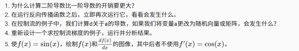
2.5.6. 练习
x.grad.zero_()
y = x**2
y.sum().backward()
x.grad
tensor([0., 2., 4., 6.])
x.grad.zero_()
x = torch.arange(40.,requires_grad=True)
y = 2 * torch.dot(x**2,torch.ones_like(x))
print(y)

y.sum().backward()
x.grad
tensor(41080., grad_fn=<MulBackward0>)


tensor([  0.,   4.,   8.,  12.,  16.,  20.,  24.,  28.,  32.,  36.,  40.,  44.,
         48.,  52.,  56.,  60.,  64.,  68.,  72.,  76.,  80.,  84.,  88.,  92.,
         96., 100., 104., 108., 112., 116., 120., 124., 128., 132., 136., 140.,
        144., 148., 152., 156.])
2.6. 概率
简单地说,机器学习就是做出预测。
根据病人的临床病史,我们可能想预测他们在下一年心脏病发作的概率
2.6.1. 基本概率论
%matplotlib inline
import torch
from torch.distributions import multinomial
from d2l import torch as d2l
投色子
fair_probs = torch.ones([6]) / 6
multinomial.Multinomial(1, fair_probs).sample()
tensor([0., 1., 0., 0., 0., 0.])
随机投十次
multinomial.Multinomial(10, fair_probs).sample()
tensor([1., 0., 4., 3., 1., 1.])
随机1000次,算每个面的概率
# 将结果存储为32位浮点数以进行除法
counts = multinomial.Multinomial(1000, fair_probs).sample()
counts / 1000  # 相对频率作为估计值
tensor([0.1650, 0.1790, 0.1750, 0.1670, 0.1490, 0.1650])
我们进行500组实验,每组抽取10个样本。
counts = multinomial.Multinomial(10, fair_probs).sample((500,))
cum_counts = counts.cumsum(dim=0)
estimates = cum_counts / cum_counts.sum(dim=1, keepdims=True)

d2l.set_figsize((6, 4.5))
for i in range(6):
    d2l.plt.plot(estimates[:, i].numpy(), label=("P(die=" + str(i + 1) + ")"))
d2l.plt.axhline(y=0.167, color='black', linestyle='dashed')
d2l.plt.gca().set_xlabel('Groups of experiments')
d2l.plt.gca().set_ylabel('Estimated probability')
d2l.plt.legend();
[外链图片转存失败,源站可能有防盗链机制,建议将图片保存下来直接上传(img-5ieNeOsC-1640697045696)(https://gitee.com/zdbya/picgo_image/raw/master/SSL_img/202112282107836.svg+xml)]
2.7. 查阅文档
2.7.1. 查找模块中的所有函数和类
import torch
print(dir(torch.distributions))
['AbsTransform', 'AffineTransform', 'Bernoulli', 'Beta', 'Binomial', 'CatTransform', 'Categorical', 'Cauchy', 'Chi2', 'ComposeTransform', 'ContinuousBernoulli', 'CorrCholeskyTransform', 'Dirichlet', 'Distribution', 'ExpTransform', 'Exponential', 'ExponentialFamily', 'FisherSnedecor', 'Gamma', 'Geometric', 'Gumbel', 'HalfCauchy', 'HalfNormal', 'Independent', 'IndependentTransform', 'Kumaraswamy', 'LKJCholesky', 'Laplace', 'LogNormal', 'LogisticNormal', 'LowRankMultivariateNormal', 'LowerCholeskyTransform', 'MixtureSameFamily', 'Multinomial', 'MultivariateNormal', 'NegativeBinomial', 'Normal', 'OneHotCategorical', 'OneHotCategoricalStraightThrough', 'Pareto', 'Poisson', 'PowerTransform', 'RelaxedBernoulli', 'RelaxedOneHotCategorical', 'ReshapeTransform', 'SigmoidTransform', 'SoftmaxTransform', 'StackTransform', 'StickBreakingTransform', 'StudentT', 'TanhTransform', 'Transform', 'TransformedDistribution', 'Uniform', 'VonMises', 'Weibull', '__all__', '__builtins__', '__cached__', '__doc__', '__file__', '__loader__', '__name__', '__package__', '__path__', '__spec__', 'bernoulli', 'beta', 'biject_to', 'binomial', 'categorical', 'cauchy', 'chi2', 'constraint_registry', 'constraints', 'continuous_bernoulli', 'dirichlet', 'distribution', 'exp_family', 'exponential', 'fishersnedecor', 'gamma', 'geometric', 'gumbel', 'half_cauchy', 'half_normal', 'identity_transform', 'independent', 'kl', 'kl_divergence', 'kumaraswamy', 'laplace', 'lkj_cholesky', 'log_normal', 'logistic_normal', 'lowrank_multivariate_normal', 'mixture_same_family', 'multinomial', 'multivariate_normal', 'negative_binomial', 'normal', 'one_hot_categorical', 'pareto', 'poisson', 'register_kl', 'relaxed_bernoulli', 'relaxed_categorical', 'studentT', 'transform_to', 'transformed_distribution', 'transforms', 'uniform', 'utils', 'von_mises', 'weibull']
2.7.2. 查找特定函数和类的用法
help(torch.ones)
Help on built-in function ones:

ones(...)
    ones(*size, *, out=None, dtype=None, layout=torch.strided, device=None, requires_grad=False) -> Tensor

    Returns a tensor filled with the scalar value `1`, with the shape defined
    by the variable argument :attr:`size`.

    Args:
        size (int...): a sequence of integers defining the shape of the output tensor.
            Can be a variable number of arguments or a collection like a list or tuple.

    Keyword arguments:
        out (Tensor, optional): the output tensor.
        dtype (:class:`torch.dtype`, optional): the desired data type of returned tensor.
            Default: if ``None``, uses a global default (see :func:`torch.set_default_tensor_type`).
        layout (:class:`torch.layout`, optional): the desired layout of returned Tensor.
            Default: ``torch.strided``.
        device (:class:`torch.device`, optional): the desired device of returned tensor.
            Default: if ``None``, uses the current device for the default tensor type
            (see :func:`torch.set_default_tensor_type`). :attr:`device` will be the CPU
            for CPU tensor types and the current CUDA device for CUDA tensor types.
        requires_grad (bool, optional): If autograd should record operations on the
            returned tensor. Default: ``False``.

    Example::

        >>> torch.ones(2, 3)
        tensor([[ 1.,  1.,  1.],
                [ 1.,  1.,  1.]])

        >>> torch.ones(5)
        tensor([ 1.,  1.,  1.,  1.,  1.])


 209
209


 被折叠的 条评论
为什么被折叠?
被折叠的 条评论
为什么被折叠?
 到【灌水乐园】发言


