


注意:本文引用自专业人工智能社区Venus AI
更多AI知识请参考原站 ([www.aideeplearning.cn])
问题描述
脑卒中是全球范围内导致成年人死亡和长期残疾的主要原因之一。它发生时,大脑部分区域因血液供应中断而缺氧,导致脑细胞死亡。早期识别脑卒中的风险因素对于预防和降低脑卒中的发生率至关重要。然而,脑卒中的风险因素多种多样,包括生活方式、遗传因素和各种健康状况。
项目目标
本项目旨在使用机器学习技术分析Brain Stroke Dataset,从而预测个体脑卒中的风险。通过构建和训练有效的预测模型,我们可以辨识高风险群体,从而提供早期干预措施。此外,该模型的建立还有助于医疗专业人士更好地理解脑卒中的各种风险因素之间的相互作用。
项目应用
- 医疗预防:为高风险群体提供个性化的预防建议。
- 公共卫生政策:协助政策制定者根据人群的风险分布制定更有效的公共卫生策略。
- 临床研究:提供研究基础,探索脑卒中发生的深层次原因。
数据集描述
Brain Stroke Dataset通常包含以下特征:
- 年龄:患者的年龄。
- 性别:患者的性别。
- 高血压:患者是否有高血压病史。
- 心脏病:患者是否有心脏病病史。
- 婚姻状况:患者的婚姻状况。
- 工作类型:患者的职业类型。
- 居住类型:患者居住的环境(城市或乡村)。
- 平均葡萄糖水平:患者的平均血糖水平。
- 体重指数(BMI):用于评估体重相对于身高的指标。
- 吸烟状况:患者的吸烟习惯。
项目模型与依赖
模型:
- 1. Decision Tree Classifier
- 2. Random Forest Classifier
- 3. SVM Classifier
- 4. XGBoost
依赖:
- matplotlib==3.7.1
- numpy==1.24.3
- pandas==2.0.2
- scikit_learn==1.2.2
- seaborn==0.13.0
项目详细代码
import os
import pandas as pd
import numpy as np
import seaborn as sns
import matplotlib.pyplot as plt
import sklearn
from sklearn.preprocessing import LabelEncoder
from sklearn.preprocessing import MinMaxScaler
from sklearn.model_selection import train_test_split
from sklearn.ensemble import  RandomForestClassifier
from sklearn.tree import DecisionTreeClassifier
from sklearn.svm import SVC
from sklearn.metrics import classification_report, f1_score, accuracy_score, confusion_matrix
from sklearn.model_selection import cross_val_score
data = pd.read_csv('brain_stroke.csv')
data.head(10)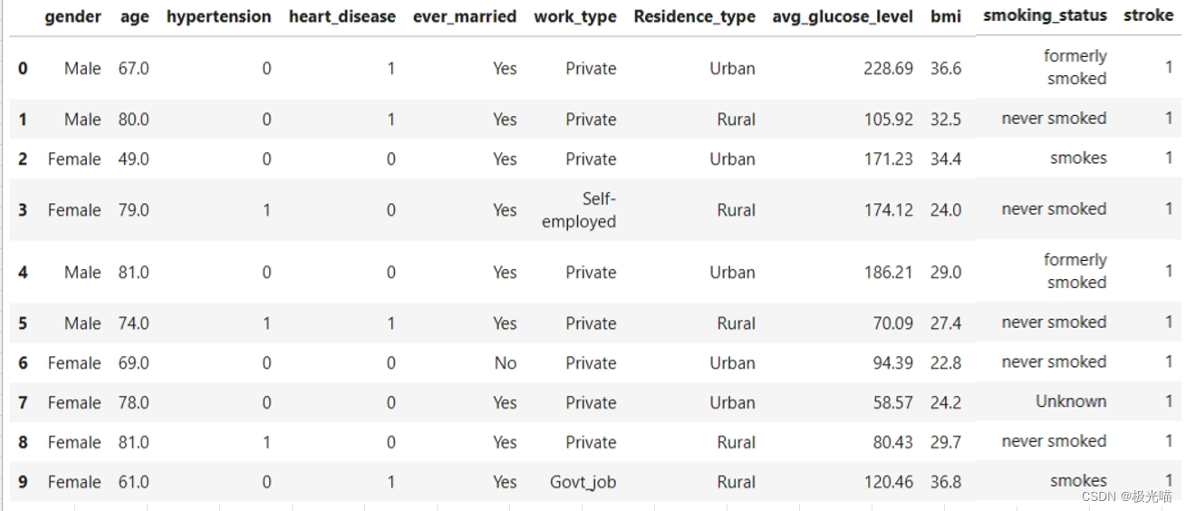
data.isna().sum()
# 数据中不存在空值
gender 0 age 0 hypertension 0 heart_disease 0 ever_married 0 work_type 0 Residence_type 0 avg_glucose_level 0 bmi 0 smoking_status 0 stroke 0 dtype: int64
data.duplicated().sum()
# 数据中不存在重复值
0
data.info()<class 'pandas.core.frame.DataFrame'> RangeIndex: 4981 entries, 0 to 4980 Data columns (total 11 columns): # Column Non-Null Count Dtype --- ------ -------------- ----- 0 gender 4981 non-null object 1 age 4981 non-null float64 2 hypertension 4981 non-null int64 3 heart_disease 4981 non-null int64 4 ever_married 4981 non-null object 5 work_type 4981 non-null object 6 Residence_type 4981 non-null object 7 avg_glucose_level 4981 non-null float64 8 bmi 4981 non-null float64 9 smoking_status 4981 non-null object 10 stroke 4981 non-null int64 dtypes: float64(3), int64(3), object(5) memory usage: 428.2+ KB
data.describe()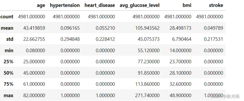
1. 探索性数据分析
-
这个数据集几乎没有经过预处理,我丢弃了异常值和非常罕见的分类值。 我还删除了“id”列。 我建议对于这个数据集,删除小于 38 岁的“年龄”特征。
-
avg_glucose_level 值的前 25% 非常高
def create_comparison_graph(feature: str, bins=2, ticks=True): fig, ax = plt.subplots(1, 2, figsize=(7,4), sharey=True, constrained_layout=True) fig.suptitle('Stroke patient based on {}'.format(feature), fontsize=16) sns.histplot(data[data['stroke'] == 0][feature], bins=bins, ax=ax[0]) ax[0].set_ylabel('Count') ax[0].set_xlabel('No Stroke') if bins == 2: ax[0].set_xticks([0,1]) if ticks: ax[0].set_xticklabels(['No', 'Yes']) sns.histplot(data[data['stroke'] == 1][feature], bins=bins, ax=ax[1]) ax[1].set_xlabel('Stroke') if bins == 2: ax[1].set_xticks([0,1]) if ticks: ax[1].set_xticklabels(['No', 'Yes']) # fig.show() # 这行可以移除,在jupyter中会自动显示sns.histplot(data=data,x="avg_glucose_level",kde=True)<Axes: xlabel='avg_glucose_level', ylabel='Count'

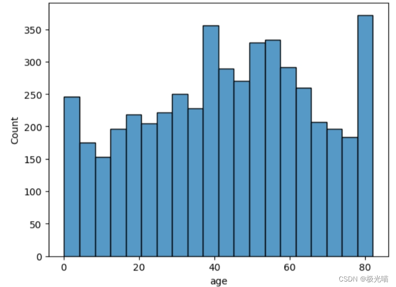
sns.histplot(data=data,x="age")
#数据很可能是从大量人群中抽取的
<Axes: xlabel='age', ylabel='Count'>
columns=data[["age","gender","stroke"]]
sns.pairplot(columns, hue="gender")
plt.show()
# 我们可以删除年龄特征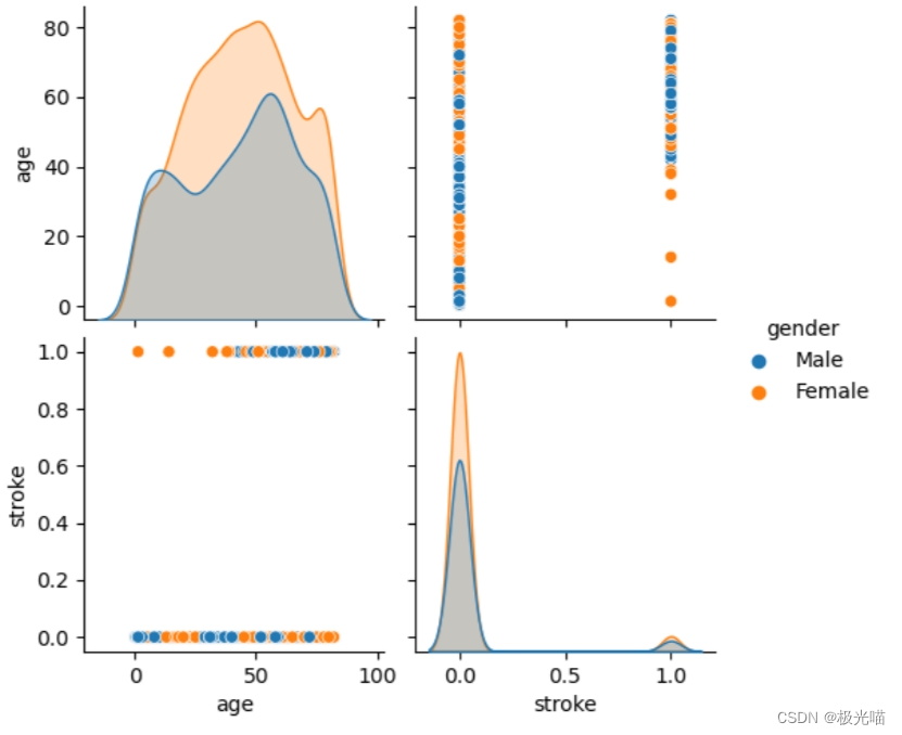
data = data.drop(["age"],axis=1)
data.head(1) 
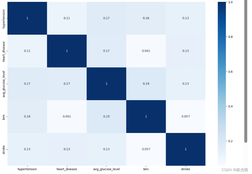
# 绘制相关性矩阵
plt.figure(figsize=(15,10))
sns.heatmap(data.corr(numeric_only=True), annot=True, cmap="Blues")
<Axes: >
#Relationship between stroke and avg_gluose_level - lower glucose level => lower chance of stroke
create_comparison_graph('avg_glucose_level',40)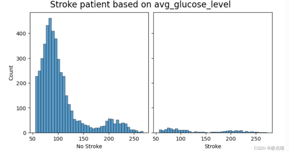
#Relationship between stroke and gender - N/A
create_comparison_graph('gender',ticks=False)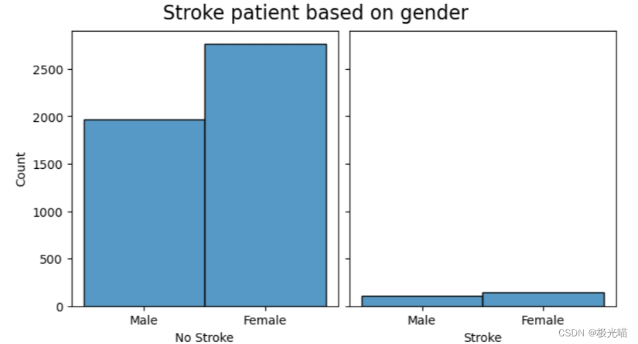
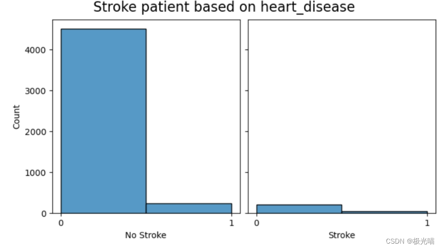
#Relationship between stroke and heart_disease - no heart disease => lower chance of getting stroke
#The conclusion is not confounding  ref: https://www.cdc.gov/stroke/risk_factors.htm#:~:text=Heart%20disease,rich%20blood%20to%20the%20brain.
create_comparison_graph('heart_disease',ticks=False)
#Relationship between stroke and work_type - confounding?
create_comparison_graph('work_type',ticks=False)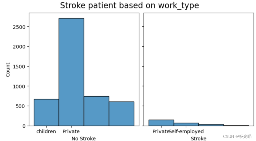
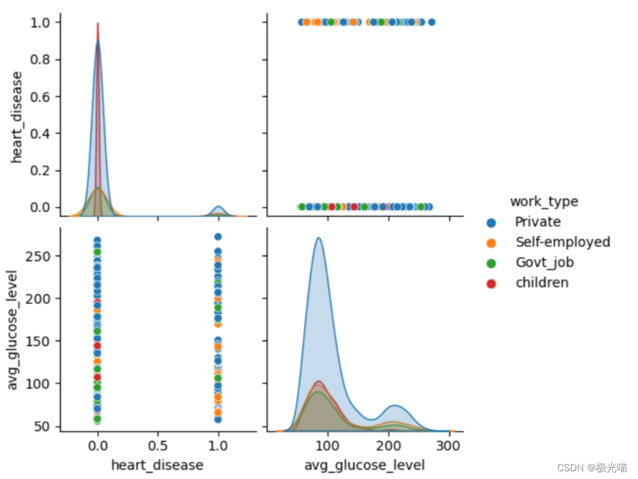
columns = data[["heart_disease","avg_glucose_level","work_type"]]
sns.pairplot(columns,hue="work_type")
plt.show()
#work_type is confounding
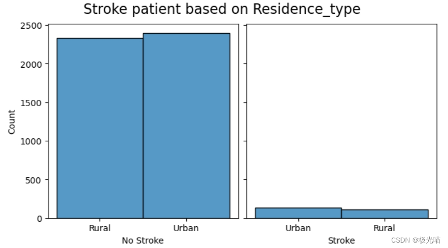
#Relationship between stroke and residence - N/A
create_comparison_graph('Residence_type',ticks=False)
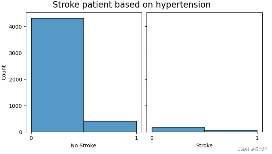
#Relationship between stroke and hypertension - lower hypertension => lower chance of stroke
create_comparison_graph('hypertension',ticks=False)
#Relationship between stroke and married status - yes
create_comparison_graph('ever_married',ticks=False)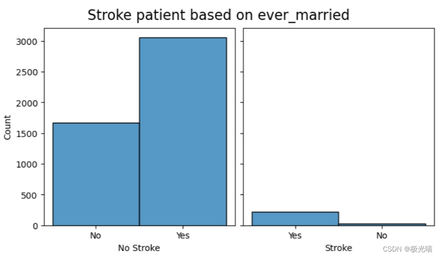
2. 训练模型
#drop gender, residence, work_type columns
data = data.drop(["gender","Residence_type","work_type"],axis=1)
data.head(1)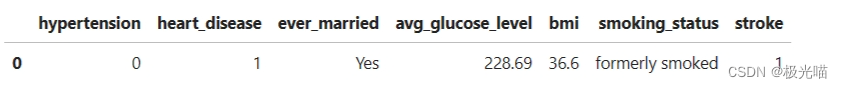
#convert non-object types to categorical values
encoder = LabelEncoder()
data['ever_married'] = encoder.fit_transform(data['ever_married'])
ever_married = {index : label for index, label in enumerate(encoder.classes_)}
data['smoking_status'] = encoder.fit_transform(data['smoking_status'])
smoking_status = {index : label for index, label in enumerate(encoder.classes_)}
x = data.drop('stroke',axis=1)
y = data['stroke']scaler = MinMaxScaler(copy=True, feature_range=(0, 1))
X = scaler.fit_transform(x)#train, test split
x_train,x_test,y_train,y_test=train_test_split(x,y,test_size=0.2,random_state=0)Decison Tree Classifier
dt = DecisionTreeClassifier(max_depth=6)
dt.fit(x_train,y_train)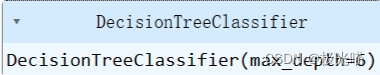
y_predict = dt.predict(x_test)print("Decision Tree Accuracy:")
print(accuracy_score(y_test,y_predict))
decision_tree_accuracy = accuracy_score(y_test,y_predict)Decision Tree Accuracy: 0.9458375125376128
from sklearn.metrics import accuracy_score, roc_auc_score, confusion_matrix
import seaborn as sns
import matplotlib.pyplot as plt
# 计算决策树的准确度
print("Decision Tree Accuracy:")
decision_tree_accuracy = accuracy_score(y_test, y_predict)
print(decision_tree_accuracy)
# 计算 ROC AUC 分数
decision_tree_roc_auc = roc_auc_score(y_test, y_predict)
print("Decision Tree ROC AUC Score:")
print(decision_tree_roc_auc)
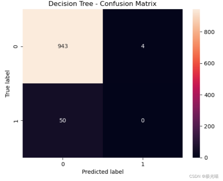
# 计算并绘制混淆矩阵
cm = confusion_matrix(y_test, y_predict)
sns.heatmap(cm, annot=True, fmt='d')
plt.title('Decision Tree - Confusion Matrix')
plt.ylabel('True label')
plt.xlabel('Predicted label')
plt.show()Decision Tree Accuracy: 0.9458375125376128 Decision Tree ROC AUC Score: 0.4978880675818374
Random Forest Classifier
rf = RandomForestClassifier()
rf.fit(x_train,y_train)
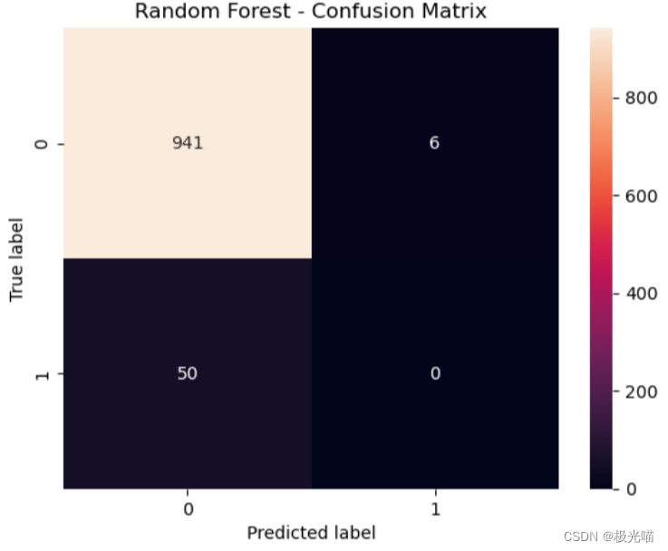
y_predict = rf.predict(x_test)# 计算随机森林的准确度
print("Random Forest Accuracy:")
decision_tree_accuracy = accuracy_score(y_test, y_predict)
print(decision_tree_accuracy)
# 计算 ROC AUC 分数
decision_tree_roc_auc = roc_auc_score(y_test, y_predict)
print("Random Forest ROC AUC Score:")
print(decision_tree_roc_auc)
# 计算并绘制混淆矩阵
cm = confusion_matrix(y_test, y_predict)
sns.heatmap(cm, annot=True, fmt='d')
plt.title('Random Forest - Confusion Matrix')
plt.ylabel('True label')
plt.xlabel('Predicted label')
plt.show()Random Forest Accuracy: 0.9438314944834504 Random Forest ROC AUC Score: 0.4968321013727561
SVM based classifier
svc = SVC(kernel='rbf', gamma=1, C=2)
svc.fit(x_train, y_train)
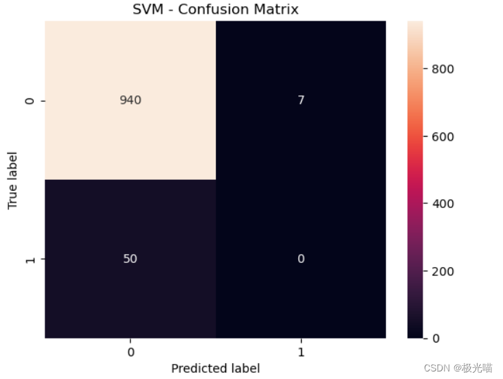
y_predict = svc.predict(x_test)# 计算随机森林的准确度
print("SVM Accuracy:")
decision_tree_accuracy = accuracy_score(y_test, y_predict)
print(decision_tree_accuracy)
# 计算 ROC AUC 分数
decision_tree_roc_auc = roc_auc_score(y_test, y_predict)
print("SVM ROC AUC Score:")
print(decision_tree_roc_auc)
# 计算并绘制混淆矩阵
cm = confusion_matrix(y_test, y_predict)
sns.heatmap(cm, annot=True, fmt='d')
plt.title('SVM - Confusion Matrix')
plt.ylabel('True label')
plt.xlabel('Predicted label')
plt.show()SVM Accuracy: 0.9428284854563691 SVM ROC AUC Score: 0.4963041182682154
XGBoost Classifier
# 计算准确度
xgboost_accuracy = accuracy_score(y_test, y_predict)
print('XGBoost Accuracy:', xgboost_accuracy)

# 计算 ROC AUC 分数
xgboost_roc_auc = roc_auc_score(y_test, y_predict)
print("XGBoost ROC AUC Score:", xgboost_roc_auc)

# 计算并绘制混淆矩阵
cm = confusion_matrix(y_test, y_predict)
sns.heatmap(cm, annot=True, fmt='d')
plt.title('XGBoost - Confusion Matrix')
plt.ylabel('True label')
plt.xlabel('Predicted label')
plt.show()
XGBoost Accuracy: 0.9428284854563691 XGBoost ROC AUC Score: 0.4963041182682154

import pandas as pd
import matplotlib.pyplot as plt

# 假设的准确度数据
accuracy_decision_tree = decision_tree_accuracy
accuracy_random_forest = random_forest_accuracy
accuracy_svc = svm_accuracy
accuracy_xgboost = xgboost_accuracy

# 准确度数据和模型名称
accuracies = [accuracy_decision_tree, accuracy_random_forest, accuracy_svc, accuracy_xgboost]
model_names = ['Decision Tree', 'Random Forest', 'SVM', 'XGBoost']

# 创建 DataFrame
accuracy_df = pd.DataFrame({'Model': model_names, 'Accuracy': accuracies})

# 显示表格
accuracy_df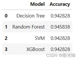


 1万+
1万+

 被折叠的 条评论
为什么被折叠?
被折叠的 条评论
为什么被折叠?
 到【灌水乐园】发言


