


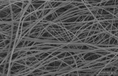
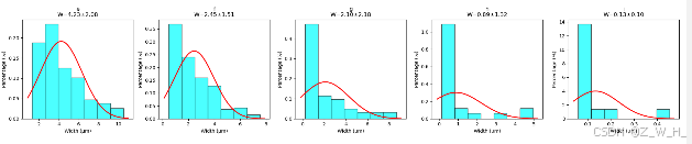
根据五张显微镜图片(11-1.tif ~ 11-5.tif),统计纤维宽度分布,并画出直方图+正态分布拟合曲线
主要步骤
- 读取图片
- 图像预处理(灰度化、二值化、去噪等)
- 边缘检测/骨架提取
- 测量纤维宽度
- 统计宽度分布,绘制直方图和正态分布拟合曲线
图片
代码
import cv2
import numpy as np
import matplotlib.pyplot as plt
from scipy.stats import norm
from skimage import measure
def measure_fiber_width(image_path, pixel_per_um):
# 读取图片
img = cv2.imread(image_path, cv2.IMREAD_GRAYSCALE)
# 二值化
_, binary = cv2.threshold(img, 0, 255, cv2.THRESH_OTSU)
# 反色(确保纤维为白色)
binary = 255 - binary
# 去噪
binary = cv2.medianBlur(binary, 5)
# 连通域分析
labels = measure.label(binary, connectivity=2)
props = measure.regionprops(labels)
widths = []
for prop in props:
# 只考虑较大的区域,过滤噪声
if prop.area > 100:
minr, minc, maxr, maxc = prop.bbox
width = max(maxr - minr, maxc - minc) / pixel_per_um
widths.append(width)
return widths
def remove_outliers(data, n_std=2):
mu = np.mean(data)
std = np.std(data)
filtered = [x for x in data if (mu - n_std*std) <= x <= (mu + n_std*std)]
return filtered
def plot_width_distribution(widths, ax, title):
widths = remove_outliers(widths, n_std=1)
# 直方图
n, bins, patches = ax.hist(widths, bins=7, color='cyan', edgecolor='black', alpha=0.7, density=True)
# 拟合正态分布
mu, std = norm.fit(widths)
xmin, xmax = ax.get_xlim()
x = np.linspace(xmin, xmax, 100)
p = norm.pdf(x, mu, std)
ax.plot(x, p, 'r-', lw=2)
ax.set_xlabel('Width (μm)')
ax.set_ylabel('Percentage (%)')
ax.set_title(f'{title}\nW={mu:.2f}±{std:.2f}')
ax.grid(False)
# 假设每像素代表的微米数(需根据标尺换算)
# pixel_per_um = 2.0 # 你需要根据图片标尺换算
file_list = ['11-1.tif', '11-2.tif', '11-3.tif', '11-4.tif', '11-5.tif']
titles = ['e', 'f', 'g', 'h', 'i']
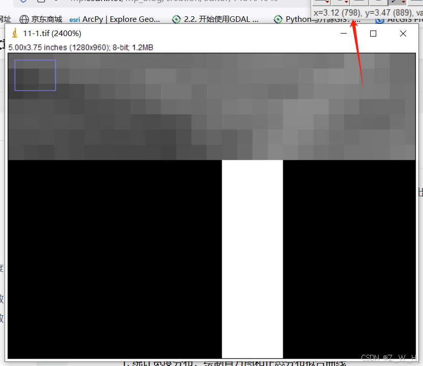
pixel_per_ums = [(1255-798)/50.0,(1255-748)/20.0,(1255-748)/10.0,(1255-798)/5.0,(1255-849)/2.0]
fig, axs = plt.subplots(1, 5, figsize=(20, 4))
for i, (file, title,pixel_per_um) in enumerate(zip(file_list, titles,pixel_per_ums)):
widths = measure_fiber_width(file, pixel_per_um)
plot_width_distribution(widths, axs[i], title)
plt.tight_layout()
plt.show()
结果
注意
- pixel_per_um 需要你根据图片标尺自行换算(如50μm对应多少像素)。
步骤
1.在图片中找到标尺
比如图片上有一条标注为“50 μm”的标尺。
2.用图像软件测量标尺长度(像素)
用如 ImageJ、Photoshop、画图、或 Python 脚本等工具,测量这条标尺在图片中占多少像素(比如 200 像素)。
3.计算每微米对应的像素数
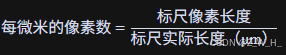
例如:标尺为 50 μm,测得长度为 200 像素,则
![]()
也就是 1 μm = 4 像素。
4.计算每像素对应的微米数(pixel_per_um)
你的代码需要的是“每像素对应的微米数”,即
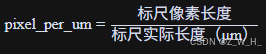
你的代码里 pixel_per_um 实际上是“每微米多少像素”,所以用第一个公式。
ImageJ
起始像素
结束像素
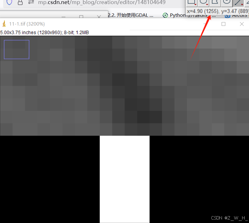


 854
854

 被折叠的 条评论
为什么被折叠?
被折叠的 条评论
为什么被折叠?
 到【灌水乐园】发言


