


文章目录
论文简介
一、提出新的全卷积神经网络(Fully Convolutional Network, FCN)U-Net,并指出其在ISBI挑战赛的表现要优于之前所有采用滑动窗口的卷积网络(a sliding-window convolutional network)
二、新提出的U-Net网络利用Encoder-Decoder的方式(原文描述为:The architecture consists of a contracting path to capture context and a symmetric expanding path that enables precise localization,该网络结构由捕获上下文的收缩路径和实现精确定位的对称扩展路径组成)可以从很少的图像进行端到端的训练
三、由于是全卷积网络,需要训练的参数则是每一层的卷积核,因此整个网络的模型参数并不庞大,这也是原文中描述U-Net网络快的原因,在6G显存的GPU就能进行良好的训练,整个网络训练采用Caffe框架
四、应用于医学领域,考虑与许多传统视觉领域的不同应用场景,指出在生物医学图像处理中,期望的输出应该包括定位,即应该为每个像素分配类别标签
五、对标Ciresan 《Deep neural networks segment neuronal membranes in electron microscopy images》等人使用滑动窗口的神经网络,指出滑动窗口神经网络其存在的缺点以及本文提出的U-Net的改进之处
论文研读
Ciresan工作的不足
Ciresan等人使用滑动窗口的方式(sliding-window convolutional network)设计并训练了一个网络,通过提供围绕该像素的局部区域(补丁,patch)作为输入来预测每个像素的类别标签
优点:1.该网络可以对像素进行定位
2.由于使用补丁(patch)的方式,训练数据远大于训练图像的数量,这使得最终网络在ISBI 2012上大幅度赢得了EM细分挑战
缺点:1.由于网络必须针对每个patch单独,这导致网络运行非常的慢
2由于截取了大量的patch不同patch之间存在的重合部分大大提升了数据的冗余信息,并且较大的patch需要更多的max-pooling层,这会降低定位的准确率,而较小的patch包括的信息较少,能够查看到的上下文信息较少
U-Net 中 overlap tile策略
原文中描述如下:
The network does not have any fully connected layers and only uses the valid part of each convolution, i.e., the segmentation map only contains the pixels, for which the full context is available in the input image. This strategy allows the seamless segmentation of arbitrarily large images by an overlap-tile strategy (see Figure 2). To predict the pixels in the border region of the image, the missing context is extrapolated by mirroring the input image. This tiling strategy is important to apply the network to large images, since otherwise the resolution would be limited by the GPU memory.
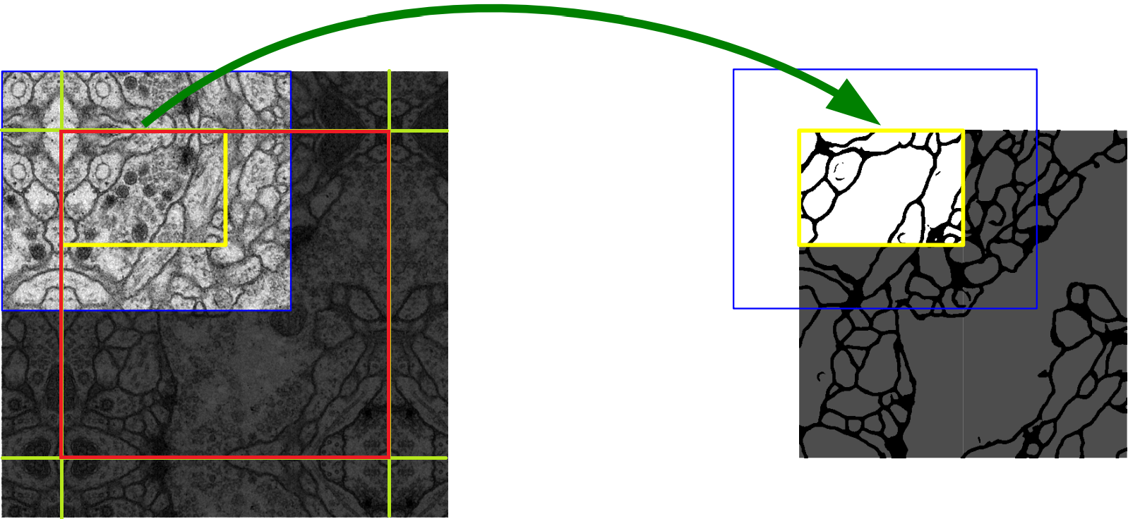
该策略的思想是:对图像的某一块像素点(黄框内部分)进行预测时,需要该图像块周围的像素点(蓝色框内)提供上下文信息(context),以获得更准确的预测
这样的策略会带来一个问题,图像边界的图像块没有周围像素,因此作者对周围像素采用了镜像扩充。我对论文中的图片进行了编辑,下图中红框部分为原始图片即对应到右边的整张图片,绿色直线为镜像的边界,其周围扩充的像素点均由原图沿绿色线对称得到。这样,边界图像块也能得到准确的预测。但这会导致另一个问题,这样的操作会带来图像重叠问题,即第一块图像周围的部分会和第二块图像重叠。因此作者在卷积时只使用有效部分(valid part of each convolution),虽然卷积的时候会用到周围的像素点(蓝色框内),但最终传到下一层的只有中间原先图像块(黄色框内)的部分
FCN的优点
《Fully convolutional networks for semantic segmentation》中的主要思想是通过连续的层来补充通常的收缩网络,其中池化运算(pooling)被上采样运算(upsampling)代替。 显然的,通过上采样操作讲增加输出的分辨率。 为了定位,将收缩路径中的高分辨率特征与上采样的输出结合在一起。 然后,连续的卷积层可以根据此信息学习组装更精确的输出
U-Net网络结构

如上图所示,U-Net的网络命名明显来源于其U型的网络结构,在这里我们利用Encoder-Decoder替换原文所描述的(收缩路径,contracting path)-(扩张路径,expanding path)
一、U-Net在Encoder部分使用的valid part of each convolution,即U-Net采用valid模式的卷积,这使得每一次卷积后,图像的尺寸发生变化
二、U-Net在Decoder部分采用Up-Cov即反卷积操作,使得每一次Up-Cov后的特征图尺寸都是上一个特征图尺寸的二倍
三、对于同一楼层的Encoder与Decoder,两者的特征图尺寸在宽高处不同,论文中采用剪裁的方式,将同一楼层的Encoder特征图从中心剪裁出与Decoder楼层相同尺寸的特征图,然后进行concat(特征图通道拼接),最终输入segmentation map
总结:U-Net在同一楼层采用Valid Conv+ReLU的方式提取特征,采用Max Pooling方式在下一楼层将特征图尺寸缩小为原来的
1
2
\frac{{\text{1}}}{{\text{2}}}
21,通过Crop操作将Encoder的特征图尺寸裁剪到同一楼层的Decoder大小再通过concat操作连接Encoder与Decoder同一楼层的特征图获得最终的输入特征图
训练方式
训练参数设置
论文中采用的是SGD(stochastic gradient descent,随机梯度下降实现的网络)。比起输入较大的batch size,作者更倾向于使用较大的输入尺寸(或者分片,即论文中所描述的tile),训练时采用的momentum参数为0.99
损失函数定义
softmax定义:
p
(
x
)
=
e
a
k
(
x
)
∑
k
′
=
1
K
e
a
k
′
(
x
)
p(x) = \frac{{{e^{{a_k}(x)}}}}{{\sum\nolimits_{{k^′} = 1}^K {{e^{{a_{{k^′}}}(x)}}} }}
p(x)=∑k′=1Keak′(x)eak(x)
其中
a
k
(
x
)
{a_k}(x)
ak(x)表示特征通道
k
k
k像素位置
x
x
x的激活值,
K
K
K表示类别数,
p
k
(
x
)
{p_k}(x)
pk(x)是估计最大值函数。即
p
k
(
x
)
≈
1
{p_k}(x)\approx1
pk(x)≈1对于
k
k
k来说具有最大的
a
k
(
x
)
{a_k}(x)
ak(x),对于其它所有
k
k
k的取值,
p
k
(
x
)
≈
0
{p_k}(x)\approx0
pk(x)≈0
cross entropy定义:
E
=
∑
x
∈
Ω
w
(
x
)
log
(
p
l
(
x
)
(
x
)
)
E = \sum\limits_{x \in \Omega } {w(x)\log ({p_{l(x)}}(x))}
E=x∈Ω∑w(x)log(pl(x)(x))
通过交叉惩罚每个位置的
p
l
(
x
)
(
x
)
p_{l(x)}(x)
pl(x)(x)与
1
1
1的偏差,其中
l
:
Ω
→
{
1
,
.
.
.
,
K
}
l: \Omega \to\left\{ {1,...,K} \right\}
l:Ω→{1,...,K} 是每个像素的真实标签值,
w
:
Ω
→
R
w: \Omega \to R
w:Ω→R 是引入的权重图以使得某些像素在训练中更加重要
初始化权重方法
我们为每个ground truth segmentation(即图片对应的label)预先计算权重图,以补偿训练数据集中某类像素的不同频率,并迫使网络学习我们在相互的细胞间引入的分隔边界,如下图c,d所示。【简而言之就是通过计算一个预先的权重图,迫使网络训练能更好的分割清细胞间隙,因为生物医学图中很多细胞靠得很近,呈现一种紧挨的状态】

使用形态学运算来计算分离边界。然后使用如下公式计算权重图
w
(
x
)
=
w
c
(
x
)
+
w
0
•
exp
(
−
(
d
1
(
x
)
+
d
2
(
x
)
)
2
2
σ
2
)
w(x) = {w_c}(x) + {w_0}•\exp ( - \frac{{{{({d_1}(x) + {d_2}(x))}^2}}}{{2{\sigma ^2}}})
w(x)=wc(x)+w0•exp(−2σ2(d1(x)+d2(x))2)
其中 w c : Ω → R w_c: \Omega \to R wc:Ω→R是用于平衡每个类频率的权重图, d 1 : Ω → R d_1: \Omega \to R d1:Ω→R表示到最近一个细胞边界的距离,而 d 2 : Ω → R d_2: \Omega \to R d2:Ω→R表示到第二个最近细胞边界的距离。在我们的实验中,我们设置 w 0 = 10 w_0 = 10 w0=10, σ ≈ 5 σ≈5 σ≈5像素
在具有许多卷积层和不同路径的深度网络中,权重的良好初始化非常重要。否则,网络的某些部分可能会过度激活,而其它部分则永远不会起作用。理想情况下,应调整初始权重使网络中的每个特征图都具有大致的单位方差。对于具有我们这种架构(依次卷积和ReLU层)的网络,可以通过从具有标准偏差 2 / N \sqrt{2 / N} 2/N的高斯分布中提取初始权重来实现,其中N表示一个神经元引入的节点数。例如,对于上一层的 3 x 3 3x3 3x3卷积和 64 个 64个 64个特征通道, N = 9 ⋅ 64 = 576 N = 9·64 = 576 N=9⋅64=576
数据增强
数据增强的目的可以从少量的训练样本中扩充训练数据,对于训练网络所需的不变性和鲁棒性至关重要,论文中作者使用的数据增强方法包括:平移、旋转、形变、灰度变换。最关键的是U-Net论文使用了随机弹性形变并指出随机弹性形变对于使用少量标注样本训练分割网络是一个非常关键的概念,原文中对此的解释是:在生物医学组织中,变形是组织中最常见的变化,随机弹性形变可以有效地模拟实际变形
随机弹性形变实现细节:
我们在粗略的3x3网格上使用随机位移矢量生成平滑变形。位移是从具有10个像素标准偏差的高斯分布中采样而来。然后使用双立方插值法计算每个像素的位移。Encoder末端的dropout层执行进一步的隐式数据增强
实验
作者展示了U-Net在三种不同分割任务中的应用。第一个任务是分割电子显微镜下的神经元结构。下图显示了数据集和获得的分割的一个例子
训练数据是一组30幅图像(512×512像素),来自果蝇第一龄幼虫腹侧神经索(VNC)的连续切片透射电子显微镜。每幅图像都有一个相应的完全注释的细胞(白色)和膜(黑色)的基础事实分割图。测试集是公开的,但它的分割图是保密的。可以通过将预测的膜概率图(membrane probability map)发送给组织者来获得评估。评估是通过对10个不同级别的map(即前面的膜概率图,membrane probability map)进行阈值处理,并计算“warping error”,“Rand error”以及“pixel error”来完成
U-Net(7个旋转版本输入数据的平均值)在没有任何进一步的预处理或后处理的情况下实现了0.0003529的“warping error”(新的最佳分数)和0.0382的“Rand error”,具体数据参见下表

这比Ciresan等人的滑动窗口卷积网络结果要好得多,其最佳提交的“warping error”为0.000420,“Rand error”为0.0504。 就“Rand error”而言,在此数据集上唯一表现更好的算法是使用适用于Ciresan概率图的高度数据集特定后处理方法
除此之外,作者还将U-Net应用于光显微图像中的细胞分割任务。这项分离任务是2014年和2015年ISBI细胞追踪挑战的一部分。第一个数据集“PHc-U373”包含在聚丙烯酰亚胺基底上的胶质母细胞瘤-星形细胞瘤,U373细胞,通过相差显微镜记录(见下图a,b)。它包含35个部分注释的训练图像。在这里,我们实现了92%的平均IOU(intersection over union),这明显优于排名第二83%IOU的算法(见下表)。第二个数据集“DIC-HeLa”是平板玻璃上的HeLa细胞,通过差分干涉对比显微镜记录。它包含20个部分注释的训练图像。在这里,我们实现了77.5%的平均IOU,这明显优于排名第二46%IOU的算法


结论
U-Net架构在截然不同的生物医学细分应用中实现了非常好的性能。 借助具有弹性变形的数据增强功能,它仅需要很少的带注释的图像,并且在NVidia Titan GPU(6 GB)上只有10小时的非常合理的训练时间。 我们提供完整的基于Caffe的实施和训练有素的网络。 我们确信U-Net架构可以轻松地应用于更多任务
补充
滑动窗口卷积网络
滑动窗口卷积网络(sliding-window convolutional network):在目标检测问题中,我们通常必须找到图像中所有可能的目标,例如图像中的所有汽车,图像中的所有行人,图像中的所有自行车等。为了实现这一点,我们使用一种名叫滑动窗口检测的算法
•在此算法中,我们选择特定大小的网格单元,例如我们选择大小为2x2的网格单元
•我们使上面的网格单元穿过图像,并在网格单元中对图像的一部分进行卷积并预测输出
•然后,我们将网格单元滑过第2步,然后对图像的下一部分进行卷积
•这样,我们就覆盖了整个图像。
•我们对不同的网格单元大小重复相同的过程

滑动窗的缺点:
这在计算上很昂贵(使用了较简单的线性分类器,与神经网络相比,该分类器的计算成本并不高)
耗时长
为了解决这样的缺点,我们将卷积与其结合就构成了滑动窗口卷积网络,这种方法在Yolo系列广泛运用,具体这里不在赘述,可参考百度架构师手把手教深度学中课节4: 深度学习实践应用:计算机视觉→目标检测,除了Yolo,Faster Rcnn中的anchor也是利用了滑动窗口+卷积的方式
U-Net实现
论文中U-Net代码实现paper_unet.py,直接在终端运行python paper_unet.py将会打印各层的维度
import numpy as np
import paddle
import paddle.fluid as fluid
from paddle.fluid.dygraph import to_variable
from paddle.fluid.dygraph import Layer
from paddle.fluid.dygraph import Conv2D
from paddle.fluid.dygraph import BatchNorm
from paddle.fluid.dygraph import Pool2D
from paddle.fluid.dygraph import Conv2DTranspose


class Encoder(Layer):
    def __init__(self, num_channels, num_filters):
        super(Encoder, self).__init__()
        #TODO: encoder contains:
        #       1 3x3conv + 1bn + relu +
        #       1 3x3conc + 1bn + relu +
        #       1 2x2 pool
        # return features before and after pool
        self.conv1 = Conv2D(num_channels,
                            num_filters,
                            filter_size=3,
                            stride=1,
                            padding=0)
        self.bn1 = BatchNorm(num_filters, act='relu')

        self.conv2 = Conv2D(num_filters,
                            num_filters,
                            filter_size=3,
                            stride=1,
                            padding=0)
        self.bn2 = BatchNorm(num_filters, act='relu')

        self.pool = Pool2D(pool_size=2, pool_stride=2, pool_type='max', ceil_mode=True)


    def forward(self, inputs):
        # TODO: finish inference part
        x = self.conv1(inputs)
        x = self.bn1(x)
        x = self.conv2(x)
        x = self.bn2(x)
        x_pooled = self.pool(x)

        return x, x_pooled


class Decoder(Layer):
    def __init__(self, num_channels, num_filters):
        super(Decoder, self).__init__()
        # TODO: decoder contains:
        #       1 2x2 transpose conv (makes feature map 2x larger)
        #       1 3x3 conv + 1bn + 1relu +
        #       1 3x3 conv + 1bn + 1relu
        self.up = Conv2DTranspose(num_channels=num_channels,
                                  num_filters=num_filters,
                                  filter_size=2,
                                  stride=2)

        self.conv1 = Conv2D(num_channels,
                            num_filters,
                            filter_size=3,
                            stride=1,
                            padding=0)
        self.bn1 = BatchNorm(num_filters, act='relu')

        self.conv2 = Conv2D(num_filters,
                            num_filters,
                            filter_size=3,
                            stride=1,
                            padding=0)
        self.bn2 = BatchNorm(num_filters, act='relu')

    def forward(self, inputs_prev, inputs):

        # TODO: forward contains an Pad2d and Concat
        x = self.up(inputs)

        x = fluid.layers.concat([inputs_prev, x], axis=1)
        x = self.conv1(x)
        x = self.bn1(x)
        x = self.conv2(x)
        x = self.bn2(x)

        return x


class UNet(Layer):
    def __init__(self, num_classes=59):
        super(UNet, self).__init__()
        # encoder: 3->64->128->256->512
        # mid: 512->1024->1024

        #TODO: 4 encoders, 4 decoders, and mid layers contains 2 1x1conv+bn+relu
        self.down1 = Encoder(num_channels=3, num_filters=64)
        self.down2 = Encoder(num_channels=64, num_filters=128)
        self.down3 = Encoder(num_channels=128, num_filters=256)
        self.down4 = Encoder(num_channels=256, num_filters=512)

        self.mid_conv1 = Conv2D(512, 1024, filter_size=3, padding=0, stride=1)
        self.mid_bn1 = BatchNorm(1024, act='relu')
        self.mid_conv2 = Conv2D(1024, 1024, filter_size=3, padding=0, stride=1)
        self.mid_bn2 = BatchNorm(1024, act='relu')

        self.up4 = Decoder(1024, 512)
        self.up3 = Decoder(512, 256)
        self.up2 = Decoder(256, 128)
        self.up1 = Decoder(128, 64)

        self.last_conv = Conv2D(num_channels=64, num_filters=num_classes, filter_size=1)

    def forward(self, inputs):
        x1, x = self.down1(inputs)
        print(x1.shape, x.shape)
        x2, x = self.down2(x)
        print(x2.shape, x.shape)
        x3, x = self.down3(x)
        print(x3.shape, x.shape)
        x4, x = self.down4(x)
        print(x4.shape, x.shape)
        # middle layers
        x = self.mid_conv1(x)
        x = self.mid_bn1(x)
        x = self.mid_conv2(x)
        x = self.mid_bn2(x)

        x4 = fluid.layers.crop_tensor(x4, shape=[1, 512, 56, 56], offsets=[0, 0, 4, 4], name=None)
        x = self.up4(x4, x)
        x3 = fluid.layers.crop_tensor(x3, shape=[1, 256, 104, 104], offsets=[0, 0, 16, 16], name=None)
        print(x3.shape, x.shape)
        x = self.up3(x3, x)
        x2 = fluid.layers.crop_tensor(x2, shape=[1, 128, 200, 200], offsets=[0, 0, 40, 40], name=None)
        print(x2.shape, x.shape)
        x = self.up2(x2, x)
        print(x1.shape, x.shape)
        x1 = fluid.layers.crop_tensor(x1, shape=[1, 64, 392, 392], offsets=[0, 0, 88, 88], name=None)
        x = self.up1(x1, x)
        print(x.shape)

        x = self.last_conv(x)

        return x


def main():
    with fluid.dygraph.guard(fluid.CPUPlace()):
        model = UNet(num_classes=2)
        x_data = np.random.rand(1, 3, 572, 572).astype(np.float32)
        inputs = to_variable(x_data)
        pred = model(inputs)

        print(pred.shape)


if __name__ == "__main__":
    main()
输入结果

具体网络结构解析以及代码敲写参考图像分割7日打卡营


 2792
2792


 被折叠的 条评论
为什么被折叠?
被折叠的 条评论
为什么被折叠?
 到【灌水乐园】发言


