使用Tensor及Autograd实现机器学习

使用Tensor及Autograd实现机器学习

表达式：$y=3x^2+2$

模型：$y=w{x}^2+b$

损失函数：$Loss=\frac{1}{2}{\sum }_{i=1}^{100}(w{x}_i^2+b-y_i{)}^2$

对损失函数求导：
$\frac{\partial Loss}{\partial w}={\sum }_{i=1}^{100}(w{x}_i^2+b-y_i{)}^2{x}_i^2$

$\frac{\partial Loss}{\partial b}={\sum }_{i=1}^{100}(w{x}_i^2+b-y_i{)}^2$

利用梯度下降法学习参数，学习率为:lr

$w_1-=lr\ast \frac{\partial Loss}{\partial w}$

$b_1-=lr\ast \frac{\partial Loss}{\partial b}$

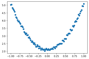
1.生成训练数据

import torch
from matplotlib import pyplot as plt

torch.manual_seed(100)
dtype = torch.float
# 生成x坐标数据，x为tensor，转成100x1的形状
# dim = 1表示列
x = torch.unsqueeze(torch.linspace(-1, 1, 100), dim=1)
# print(x)
# 生成y坐标数据，y为tensor，100x1的形状，并且加一点噪声
y = 3*x.pow(2)+2 + 0.2*torch.rand(x.size())
# 把tensor转成numpy画图
plt.scatter(x.numpy(), y.numpy())
plt.show()

2.初始化权重参数

torch.rand和torch.randn有什么区别？

• torch.rand均匀分布，torch.randn是标准正态分布。

# 随即初始化参数，参数w,b是需要学习的，所以requires_grad=True

w = torch.randn(1, 1, dtype=dtype, requires_grad=True)
# print(w)
b = torch.zeros(1, 1, dtype=dtype, requires_grad=True)
# print(b)

tensor([[0.]], requires_grad=True)

3.训练模型

lr = 0.001
for i in range(8000):
    # 前向传播 mm()矩阵乘法
    y_pred = x.pow(2).mm(w)+b
    # 损失函数
    loss = 0.5*(y_pred-y)**2
    loss = loss.sum()

    # 自动计算梯度
    loss.backward()
    # 手动更新参数，需要使用torch.no_grad()包围，使上下文中切断自动求导的计算
    with torch.no_grad():
        w -= lr*w.grad
        b -= lr*b.grad
        # 梯度清零
        w.grad.zero_()
        b.grad.zero_()

4.可视化训练结果

plt.plot(x.numpy(), y_pred.detach().numpy(), 'r-', label='predict')
# 调用detach()不再计算张量梯度
plt.scatter(x.numpy(), y.numpy(), color='blue', marker='o', label='true')
plt.xlim(-1, 1)
plt.ylim(2, 6)
plt.legend()
plt.show()
# 预测结果
print(w, b)

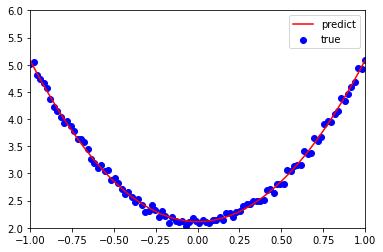
tensor([[2.9668]], requires_grad=True) tensor([[2.1138]], requires_grad=True)