使用字符级 RNN 对名称进行分类

使用字符级 RNN 对名称进行分类

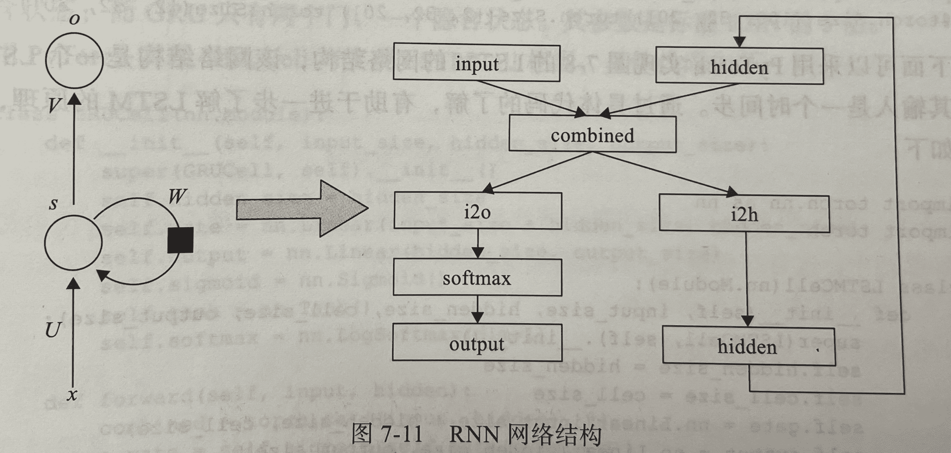
字符级 RNN 将单词读取为一系列字符，在每一步输出预测和隐藏状态，将其先前的隐藏状态输入到下一时间步。将最终预测作为输出，即单词属于哪个类。

具体来说，我们将训练来自 18 种起源语言的数千个姓氏，并根据拼写预测名称来自哪种语言：
示例：

    $ python predict.py Hinton
    (-0.47) Scottish
    (-1.52) English
    (-3.57) Irish

    $ python predict.py Schmidhuber
    (-0.19) German
    (-2.48) Czech
    (-2.68) Dutch

Note:
Download the data from
here <https://download.pytorch.org/tutorial/data.zip>_
and extract it to the current directory.

Included in the data/names directory are 18 text files named as
“[Language].txt”. Each file contains a bunch of names, one name per
line, mostly romanized (but we still need to convert from Unicode to
ASCII).

We’ll end up with a dictionary of lists of names per language,
{language: [names ...]}. The generic variables “category” and “line”
(for language and name in our case) are used for later extensibility.

from __future__ import unicode_literals, print_function, division
from io import open
import glob
import os

def findFiles(path): return glob.glob(path)

print(findFiles('data/names/*.txt'))

import unicodedata
import string

# 生成单词列表all_letters，后续one-hot编码中用来查找索引
all_letters = string.ascii_letters + " .,;'"
# n_letters 字符总数
n_letters = len(all_letters)

# Turn a Unicode string to plain ASCII, thanks to https://stackoverflow.com/a/518232/2809427
def unicodeToAscii(s):
    return ''.join(
        c for c in unicodedata.normalize('NFD', s)
        if unicodedata.category(c) != 'Mn'
        and c in all_letters
    )

print('\nunicodeToAscii:')
print(unicodeToAscii('Ślusàrski'))

# Build the category_lines dictionary, a list of names per language
category_lines = {}
all_categories = []

# Read a file and split into lines
def readLines(filename):
    lines = open(filename, encoding='utf-8').read().strip().split('\n')
    return [unicodeToAscii(line) for line in lines]

for filename in findFiles('data/names/*.txt'):
    category = os.path.splitext(os.path.basename(filename))[0]
# os.path.splitext 分割文件名和扩展名
# os.path.basename 返回文件名
    all_categories.append(category)
    lines = readLines(filename)
    category_lines[category] = lines
print()
# print(category_lines)
n_categories = len(all_categories)
print(n_categories)

['data/names/Czech.txt', 'data/names/German.txt', 'data/names/Arabic.txt', 'data/names/Japanese.txt', 'data/names/Chinese.txt', 'data/names/Vietnamese.txt', 'data/names/Russian.txt', 'data/names/French.txt', 'data/names/Irish.txt', 'data/names/English.txt', 'data/names/Spanish.txt', 'data/names/Greek.txt', 'data/names/Italian.txt', 'data/names/Portuguese.txt', 'data/names/Scottish.txt', 'data/names/Dutch.txt', 'data/names/Korean.txt', 'data/names/Polish.txt']

unicodeToAscii:
Slusarski

18

得到category_lines字典后，查看样例数据

print(category_lines['Italian'][:5])

['Abandonato', 'Abatangelo', 'Abatantuono', 'Abate', 'Abategiovanni']

把名字转换成 Tensors

为了表示单个字母，使用one-hot向量。除了当前字母的索引处为1外，其余用0填充，例如"b" = <0 1 0 0 0 ...>

为了创建一个单词，我们将一堆单词连接到一个 2D 矩阵中。<line_length x 1 x n_letters>

额外的 1 维是因为 PyTorch 假设一切都是批量的，在这里使批量大小1。

import torch
print(all_letters)
# Find letter index from all_letters, e.g. "a" = 0
def letterToIndex(letter):
    return all_letters.find(letter)

# Just for demonstration, turn a letter into a <1 x n_letters> Tensor
def letterToTensor(letter):
    tensor = torch.zeros(1, n_letters)
#     print(tensor)
    tensor[0][letterToIndex(letter)] = 1
    return tensor

# Turn a line into a <line_length x 1 x n_letters>,
# or an array of one-hot letter vectors
def lineToTensor(line):
    tensor = torch.zeros(len(line), 1, n_letters)
    for li, letter in enumerate(line):
        tensor[li][0][letterToIndex(letter)] = 1
    return tensor

print(letterToTensor('a'))

print('lineToTensor\n')
print(lineToTensor('Jones').size())
print(lineToTensor('Jones'))

abcdefghijklmnopqrstuvwxyzABCDEFGHIJKLMNOPQRSTUVWXYZ .,;'
tensor([[1., 0., 0., 0., 0., 0., 0., 0., 0., 0., 0., 0., 0., 0., 0., 0., 0., 0.,
         0., 0., 0., 0., 0., 0., 0., 0., 0., 0., 0., 0., 0., 0., 0., 0., 0., 0.,
         0., 0., 0., 0., 0., 0., 0., 0., 0., 0., 0., 0., 0., 0., 0., 0., 0., 0.,
         0., 0., 0.]])
lineToTensor

torch.Size([5, 1, 57])
tensor([[[0., 0., 0., 0., 0., 0., 0., 0., 0., 0., 0., 0., 0., 0., 0., 0., 0.,
          0., 0., 0., 0., 0., 0., 0., 0., 0., 0., 0., 0., 0., 0., 0., 0., 0.,
          0., 1., 0., 0., 0., 0., 0., 0., 0., 0., 0., 0., 0., 0., 0., 0., 0.,
          0., 0., 0., 0., 0., 0.]],

        [[0., 0., 0., 0., 0., 0., 0., 0., 0., 0., 0., 0., 0., 0., 1., 0., 0.,
          0., 0., 0., 0., 0., 0., 0., 0., 0., 0., 0., 0., 0., 0., 0., 0., 0.,
          0., 0., 0., 0., 0., 0., 0., 0., 0., 0., 0., 0., 0., 0., 0., 0., 0.,
          0., 0., 0., 0., 0., 0.]],

        [[0., 0., 0., 0., 0., 0., 0., 0., 0., 0., 0., 0., 0., 1., 0., 0., 0.,
          0., 0., 0., 0., 0., 0., 0., 0., 0., 0., 0., 0., 0., 0., 0., 0., 0.,
          0., 0., 0., 0., 0., 0., 0., 0., 0., 0., 0., 0., 0., 0., 0., 0., 0.,
          0., 0., 0., 0., 0., 0.]],

        [[0., 0., 0., 0., 1., 0., 0., 0., 0., 0., 0., 0., 0., 0., 0., 0., 0.,
          0., 0., 0., 0., 0., 0., 0., 0., 0., 0., 0., 0., 0., 0., 0., 0., 0.,
          0., 0., 0., 0., 0., 0., 0., 0., 0., 0., 0., 0., 0., 0., 0., 0., 0.,
          0., 0., 0., 0., 0., 0.]],

        [[0., 0., 0., 0., 0., 0., 0., 0., 0., 0., 0., 0., 0., 0., 0., 0., 0.,
          0., 1., 0., 0., 0., 0., 0., 0., 0., 0., 0., 0., 0., 0., 0., 0., 0.,
          0., 0., 0., 0., 0., 0., 0., 0., 0., 0., 0., 0., 0., 0., 0., 0., 0.,
          0., 0., 0., 0., 0., 0.]]])

创建网络

该RNN网络有2个线性层，对输入和隐藏状态进行操作，输出后有一个 LogSoftmax层。

import torch.nn as nn

class RNN(nn.Module):
    def __init__(self, input_size, hidden_size, output_size):
        super(RNN, self).__init__()

        self.hidden_size = hidden_size #隐藏层大小

        self.i2h = nn.Linear(input_size + hidden_size, hidden_size) #输入到隐藏层的矩阵
        self.i2o = nn.Linear(input_size + hidden_size, output_size) #输入到输出的矩阵
        self.softmax = nn.LogSoftmax(dim=1)

    def forward(self, input, hidden):
        combined = torch.cat((input, hidden), 1)
        hidden = self.i2h(combined)
#         output = self.i2o(combined)
        output = self.softmax(self.i2o(combined))
        return output, hidden

    def initHidden(self):
        return torch.zeros(1, self.hidden_size)

n_hidden = 128
print(n_letters, n_hidden, n_categories)
rnn = RNN(n_letters, n_hidden, n_categories)
print(rnn.i2h)

57 128 18
Linear(in_features=185, out_features=128, bias=True)

为了运行这个网络的一个时间步长，需要传递一个输入（在我们的例子中，为当前字母的张量）和一个先前的隐藏状态（首先将其初始化为零。得到输出（每种语言的概率）和下一个隐藏状态。

input = letterToTensor('A')
hidden = torch.zeros(1, n_hidden)

output, next_hidden = rnn(input, hidden)
print(output)

tensor([[-3.0130, -2.8982, -2.9242, -2.9052, -2.8677, -2.8176, -2.9350, -2.9060,
         -2.8688, -2.9518, -2.9790, -2.9274, -2.8601, -2.8504, -2.8594, -2.8165,
         -2.8698, -2.8037]], grad_fn=<LogSoftmaxBackward>)

为了效率起见，不想为每一步都创建一个新的张量，所以将使用lineToTensor代替letterToTensor和使用切片。这可以通过预先计算批量张量来进一步优化。

input = lineToTensor('Albert')
hidden = torch.zeros(1, n_hidden)

output, next_hidden = rnn(input[0], hidden)
print(output)

tensor([[-3.0130, -2.8982, -2.9242, -2.9052, -2.8677, -2.8176, -2.9350, -2.9060,
         -2.8688, -2.9518, -2.9790, -2.9274, -2.8601, -2.8504, -2.8594, -2.8165,
         -2.8698, -2.8037]], grad_fn=<LogSoftmaxBackward>)

输出是一个张量，其中每个项目都是该类别的可能性（越高可能性越大）。<1 x n_categories>

训练

Preparing for Training

解释网络的输出：输出是每个类别的可能性。可以使用Tensor.topk获取最大值的索引：

def categoryFromOutput(output):
    top_n, top_i = output.topk(1)
#     print(top_n, top_i)
    category_i = top_i[0].item()
    return all_categories[category_i], category_i

print(categoryFromOutput(output))

('Portuguese', 13)

需要一种快速获取训练示例（名称及其语言）的方法：

import random

def randomChoice(l):
    return l[random.randint(0, len(l) - 1)]

def randomTrainingExample():
    category = randomChoice(all_categories)
    line = randomChoice(category_lines[category])
    category_tensor = torch.tensor([all_categories.index(category)], dtype=torch.long)
    line_tensor = lineToTensor(line)
    return category, line, category_tensor, line_tensor

for i in range(10):
    category, line, category_tensor, line_tensor = randomTrainingExample()
    print('category =', category, '/ line =', line)
    

category = Vietnamese / line = Ma
category = Japanese / line = Aida
category = Portuguese / line = De santigo
category = Italian / line = Piovene
category = Scottish / line = Taylor
category = Spanish / line = Benitez
category = Vietnamese / line = Quach
category = Arabic / line = Sleiman
category = Russian / line = To The First Page
category = Korean / line = Kwang 

模型训练

RNN 的最后一层是nn.LogSoftmax，所以选择损失函数nn.NLLLoss。

criterion = nn.NLLLoss()

Each loop of training will:

• Create input and target tensors
• Create a zeroed initial hidden state
• Read each letter in and Keep hidden state for next letter
• Compare final output to target
• Back-propagate
• Return the output and loss

learning_rate = 0.005 # If you set this too high, it might explode. If too low, it might not learn

def train(category_tensor, line_tensor):
    hidden = rnn.initHidden()

    rnn.zero_grad()

    for i in range(line_tensor.size()[0]):
#  line_tensor是多个字母tensor的组合列表
#  循环中更新 hidden
        output, hidden = rnn(line_tensor[i], hidden)

    loss = criterion(output, category_tensor)
    loss.backward()

    # Add parameters' gradients to their values, multiplied by learning rate
    for p in rnn.parameters():
        p.data.add_(p.grad.data, alpha=-learning_rate)

    return output, loss.item()

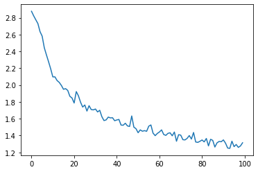
现在只需要用一堆例子来运行它。由于该 train函数返回输出和损失，我们可以打印它的预测值并绘制损失变化图。由于有 1000 个示例，我们只打印每个print_every示例，并取损失的平均值。

import time
import math

n_iters = 100000
print_every = 5000
plot_every = 1000



# Keep track of losses for plotting
current_loss = 0
all_losses = []

def timeSince(since):
    now = time.time()
    s = now - since
    m = math.floor(s / 60)
    s -= m * 60
    return '%dm %ds' % (m, s)

start = time.time()

for iter in range(1, n_iters + 1):
    category, line, category_tensor, line_tensor = randomTrainingExample()
    output, loss = train(category_tensor, line_tensor)
    current_loss += loss

    # Print iter number, loss, name and guess
    if iter % print_every == 0:
        guess, guess_i = categoryFromOutput(output)
        correct = '✓' if guess == category else '✗ (%s)' % category
        print('%d %d%% (%s) %.4f %s / %s %s' % (iter, iter / n_iters * 100, timeSince(start), loss, line, guess, correct))

    # Add current loss avg to list of losses
    if iter % plot_every == 0:
        all_losses.append(current_loss / plot_every)
        current_loss = 0

tensor([[-2.4746]], grad_fn=<TopkBackward>) tensor([[3]])
5000 5% (0m 6s) 2.6255 Ventura / Japanese ✗ (Portuguese)
tensor([[-1.8169]], grad_fn=<TopkBackward>) tensor([[16]])
10000 10% (0m 13s) 3.0541 Kron / Korean ✗ (German)
tensor([[-1.0685]], grad_fn=<TopkBackward>) tensor([[4]])
15000 15% (0m 20s) 1.0685 Ming / Chinese ✓
tensor([[-1.7141]], grad_fn=<TopkBackward>) tensor([[1]])
20000 20% (0m 27s) 1.7141 Sommer / German ✓
tensor([[-1.7253]], grad_fn=<TopkBackward>) tensor([[7]])
25000 25% (0m 34s) 1.8872 Maurice / French ✗ (Irish)
tensor([[-0.1941]], grad_fn=<TopkBackward>) tensor([[3]])
30000 30% (0m 41s) 0.1941 Jukodo / Japanese ✓
tensor([[-1.1135]], grad_fn=<TopkBackward>) tensor([[2]])
35000 35% (0m 48s) 1.1135 Khouri / Arabic ✓
tensor([[-0.2534]], grad_fn=<TopkBackward>) tensor([[12]])
40000 40% (0m 55s) 0.2534 Pietri / Italian ✓
tensor([[-0.3285]], grad_fn=<TopkBackward>) tensor([[11]])
45000 45% (1m 3s) 0.3285 Panayiotopoulos / Greek ✓
tensor([[-0.7564]], grad_fn=<TopkBackward>) tensor([[4]])
50000 50% (1m 11s) 0.7564 Song / Chinese ✓
tensor([[-0.6697]], grad_fn=<TopkBackward>) tensor([[12]])
55000 55% (1m 18s) 2.2053 Castellano / Italian ✗ (Spanish)
tensor([[-1.1335]], grad_fn=<TopkBackward>) tensor([[1]])
60000 60% (1m 26s) 2.1380 Nunez / German ✗ (Spanish)
tensor([[-1.0437]], grad_fn=<TopkBackward>) tensor([[3]])
65000 65% (1m 33s) 1.0437 Ichiyusai / Japanese ✓
tensor([[-0.9454]], grad_fn=<TopkBackward>) tensor([[12]])
70000 70% (1m 40s) 1.7417 Cardozo / Italian ✗ (Portuguese)
tensor([[-1.5786]], grad_fn=<TopkBackward>) tensor([[1]])
75000 75% (1m 47s) 2.0613 Macclelland / German ✗ (Irish)
tensor([[-0.9435]], grad_fn=<TopkBackward>) tensor([[16]])
80000 80% (1m 55s) 0.9435 Ri / Korean ✓
tensor([[-1.7442]], grad_fn=<TopkBackward>) tensor([[14]])
85000 85% (2m 3s) 2.6989 Bran / Scottish ✗ (Irish)
tensor([[-1.1392]], grad_fn=<TopkBackward>) tensor([[7]])
90000 90% (2m 11s) 1.1392 Victor / French ✓
tensor([[-0.8626]], grad_fn=<TopkBackward>) tensor([[5]])
95000 95% (2m 19s) 0.8626 Ton / Vietnamese ✓
tensor([[-0.7950]], grad_fn=<TopkBackward>) tensor([[14]])
100000 100% (2m 28s) 4.5470 Budny / Scottish ✗ (Polish)

Plotting the Results

Plotting the historical loss from all_losses shows the network
learning:

import matplotlib.pyplot as plt
import matplotlib.ticker as ticker

plt.figure()
plt.plot(all_losses)

[<matplotlib.lines.Line2D at 0x7fbbb7b60f10>]

Evaluating the Results

To see how well the network performs on different categories, we will
create a confusion matrix, indicating for every actual language (rows)
which language the network guesses (columns). To calculate the confusion
matrix a bunch of samples are run through the network with
evaluate(), which is the same as train() minus the backprop.

为了查看网络在不同类别上的表现如何，我们将创建一个混淆矩阵，actual language (rows)，the network guesses (columns)。运行 evaluate()计算混淆矩阵，这与train()减去反向传播相同。

# Keep track of correct guesses in a confusion matrix
confusion = torch.zeros(n_categories, n_categories)
n_confusion = 10000

# Just return an output given a line
def evaluate(line_tensor):
    hidden = rnn.initHidden()

    for i in range(line_tensor.size()[0]):
        output, hidden = rnn(line_tensor[i], hidden)

    return output

# Go through a bunch of examples and record which are correctly guessed
for i in range(n_confusion):
    category, line, category_tensor, line_tensor = randomTrainingExample()
    output = evaluate(line_tensor)
    guess, guess_i = categoryFromOutput(output)
    category_i = all_categories.index(category)
    confusion[category_i][guess_i] += 1

# Normalize by dividing every row by its sum
for i in range(n_categories):
    confusion[i] = confusion[i] / confusion[i].sum()

# Set up plot
fig = plt.figure()
ax = fig.add_subplot(111)
cax = ax.matshow(confusion.numpy())
fig.colorbar(cax)

# Set up axes
ax.set_xticklabels([''] + all_categories, rotation=90)
ax.set_yticklabels([''] + all_categories)

# Force label at every tick
ax.xaxis.set_major_locator(ticker.MultipleLocator(1))
ax.yaxis.set_major_locator(ticker.MultipleLocator(1))

# sphinx_gallery_thumbnail_number = 2
plt.show()

<ipython-input-61-a5b341ffc3a3>:33: UserWarning: FixedFormatter should only be used together with FixedLocator
  ax.set_xticklabels([''] + all_categories, rotation=90)
<ipython-input-61-a5b341ffc3a3>:34: UserWarning: FixedFormatter should only be used together with FixedLocator
  ax.set_yticklabels([''] + all_categories)

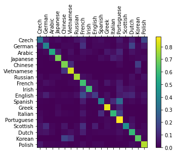
You can pick out bright spots off the main axis that show which
languages it guesses incorrectly, e.g. Chinese for Korean, and Spanish
for Italian. It seems to do very well with Greek, and very poorly with
English (perhaps because of overlap with other languages).

Running on User Input

def predict(input_line, n_predictions=3):
    print('\n> %s' % input_line)
    with torch.no_grad():
        output = evaluate(lineToTensor(input_line))

        # Get top N categories
        topv, topi = output.topk(n_predictions, 1, True)
        predictions = []

        for i in range(n_predictions):
            value = topv[0][i].item()
            category_index = topi[0][i].item()
            print('(%.2f) %s' % (value, all_categories[category_index]))
            predictions.append([value, all_categories[category_index]])

predict('Dovesky')
predict('Jackson')
predict('Satoshi')

> Dovesky
(-0.55) Russian
(-1.52) Czech
(-1.98) Polish

> Jackson
(-1.27) Scottish
(-1.61) French
(-1.83) English

> Satoshi
(-1.15) Italian
(-1.88) Portuguese
(-1.96) Polish