Seaborn 数据处理习题

1、先安装好jupyter，然后打开。、

2、完成以下问题：

Part 1

For each of the four datasets...

Compute the mean and variance of both x and y
Compute the correlation coefficient between x and y

Compute the linear regression line: y=β0+β1x+ϵy=β0+β1x+ϵ (hint: use statsmodels and look at the Statsmodels notebook)

导入所需模块和所要处理的数据：

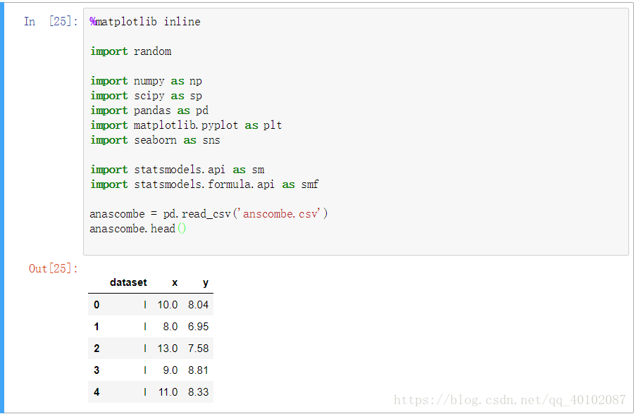
Compute the mean and variance of both x and y：

In [26]:

# 先把四个分组分离出来
anascombe_group = anascombe.groupby('dataset')
dataset_names = ['I', 'II', 'III', 'IV']

# x和y在四个分组中的均值和方差
for i in dataset_names:
    print('dataset', i, ': ')
    print('    x均值: ', anascombe_group.get_group(i)['x'].mean())
    print('    x方差: ', anascombe_group.get_group(i)['x'].var())
    print('    y均值: ', anascombe_group.get_group(i)['y'].mean())
    print('    y方差: ', anascombe_group.get_group(i)['y'].var())

Out [26]:

dataset I : 
    x均值:  9.0
    x方差:  11.0
    y均值:  7.500909090909093
    y方差:  4.127269090909091
dataset II : 
    x均值:  9.0
    x方差:  11.0
    y均值:  7.500909090909091
    y方差:  4.127629090909091
dataset III : 
    x均值:  9.0
    x方差:  11.0
    y均值:  7.500000000000001
    y方差:  4.12262
dataset IV : 
    x均值:  9.0
    x方差:  11.0
    y均值:  7.50090909090909
    y方差:  4.12324909090909

Compute the correlation coefficient between x and y:

In [27]:

# x和y的相关系数
print('相关系数：')
print(anascombe.groupby('dataset').corr())

Out [27]:

相关系数：
                  x         y
dataset                      
I       x  1.000000  0.816421
        y  0.816421  1.000000
II      x  1.000000  0.816237
        y  0.816237  1.000000
III     x  1.000000  0.816287
        y  0.816287  1.000000
IV      x  1.000000  0.816521
        y  0.816521  1.000000

Compute the linear regression line: y=β0+β1x+ϵy=β0+β1x+ϵ (hint: use statsmodels and look at the Statsmodels notebook)

In [28]:

# 线性回归方程
for i in dataset_names:
    x = anascombe_group.get_group(i)['x']
    y = anascombe_group.get_group(i)['y']
    X = sm.add_constant(x)
    model = sm.OLS(y,X)
    results = model.fit()
    print(results.summary())
    print('\nparams:', results.params, '\n\n')

Out [28]:

                            OLS Regression Results                            
==============================================================================
Dep. Variable:                      y   R-squared:                       0.667
Model:                            OLS   Adj. R-squared:                  0.629
Method:                 Least Squares   F-statistic:                     17.99
Date:                Mon, 11 Jun 2018   Prob (F-statistic):            0.00217
Time:                        13:25:48   Log-Likelihood:                -16.841
No. Observations:                  11   AIC:                             37.68
Df Residuals:                       9   BIC:                             38.48
Df Model:                           1                                         
Covariance Type:            nonrobust                                         
==============================================================================
                 coef    std err          t      P>|t|      [0.025      0.975]
------------------------------------------------------------------------------
const          3.0001      1.125      2.667      0.026       0.456       5.544
x              0.5001      0.118      4.241      0.002       0.233       0.767
==============================================================================
Omnibus:                        0.082   Durbin-Watson:                   3.212
Prob(Omnibus):                  0.960   Jarque-Bera (JB):                0.289
Skew:                          -0.122   Prob(JB):                        0.865
Kurtosis:                       2.244   Cond. No.                         29.1
==============================================================================

Warnings:
[1] Standard Errors assume that the covariance matrix of the errors is correctly specified.

params: const    3.000091
x        0.500091
dtype: float64 


                            OLS Regression Results                            
==============================================================================
Dep. Variable:                      y   R-squared:                       0.666
Model:                            OLS   Adj. R-squared:                  0.629
Method:                 Least Squares   F-statistic:                     17.97
Date:                Mon, 11 Jun 2018   Prob (F-statistic):            0.00218
Time:                        13:25:48   Log-Likelihood:                -16.846
No. Observations:                  11   AIC:                             37.69
Df Residuals:                       9   BIC:                             38.49
Df Model:                           1                                         
Covariance Type:            nonrobust                                         
==============================================================================
                 coef    std err          t      P>|t|      [0.025      0.975]
------------------------------------------------------------------------------
const          3.0009      1.125      2.667      0.026       0.455       5.547
x              0.5000      0.118      4.239      0.002       0.233       0.767
==============================================================================
Omnibus:                        1.594   Durbin-Watson:                   2.188
Prob(Omnibus):                  0.451   Jarque-Bera (JB):                1.108
Skew:                          -0.567   Prob(JB):                        0.575
Kurtosis:                       1.936   Cond. No.                         29.1
==============================================================================

Warnings:
[1] Standard Errors assume that the covariance matrix of the errors is correctly specified.

params: const    3.000909
x        0.500000
dtype: float64 


                            OLS Regression Results                            
==============================================================================
Dep. Variable:                      y   R-squared:                       0.666
Model:                            OLS   Adj. R-squared:                  0.629
Method:                 Least Squares   F-statistic:                     17.97
Date:                Mon, 11 Jun 2018   Prob (F-statistic):            0.00218
Time:                        13:25:48   Log-Likelihood:                -16.838
No. Observations:                  11   AIC:                             37.68
Df Residuals:                       9   BIC:                             38.47
Df Model:                           1                                         
Covariance Type:            nonrobust                                         
==============================================================================
                 coef    std err          t      P>|t|      [0.025      0.975]
------------------------------------------------------------------------------
const          3.0025      1.124      2.670      0.026       0.459       5.546
x              0.4997      0.118      4.239      0.002       0.233       0.766
==============================================================================
Omnibus:                       19.540   Durbin-Watson:                   2.144
Prob(Omnibus):                  0.000   Jarque-Bera (JB):               13.478
Skew:                           2.041   Prob(JB):                      0.00118
Kurtosis:                       6.571   Cond. No.                         29.1
==============================================================================

Warnings:
[1] Standard Errors assume that the covariance matrix of the errors is correctly specified.

params: const    3.002455
x        0.499727
dtype: float64 


                            OLS Regression Results                            
==============================================================================
Dep. Variable:                      y   R-squared:                       0.667
Model:                            OLS   Adj. R-squared:                  0.630
Method:                 Least Squares   F-statistic:                     18.00
Date:                Mon, 11 Jun 2018   Prob (F-statistic):            0.00216
Time:                        13:25:48   Log-Likelihood:                -16.833
No. Observations:                  11   AIC:                             37.67
Df Residuals:                       9   BIC:                             38.46
Df Model:                           1                                         
Covariance Type:            nonrobust                                         
==============================================================================
                 coef    std err          t      P>|t|      [0.025      0.975]
------------------------------------------------------------------------------
const          3.0017      1.124      2.671      0.026       0.459       5.544
x              0.4999      0.118      4.243      0.002       0.233       0.766
==============================================================================
Omnibus:                        0.555   Durbin-Watson:                   1.662
Prob(Omnibus):                  0.758   Jarque-Bera (JB):                0.524
Skew:                           0.010   Prob(JB):                        0.769
Kurtosis:                       1.931   Cond. No.                         29.1
==============================================================================

Warnings:
[1] Standard Errors assume that the covariance matrix of the errors is correctly specified.

params: const    3.001727
x        0.499909
dtype: float64 

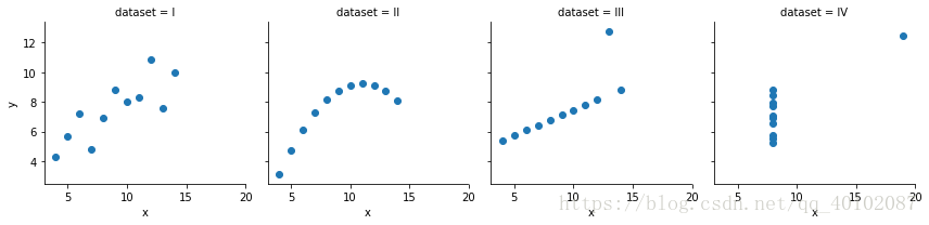
Part 2

Using Seaborn, visualize all four datasets.

hint: use sns.FacetGrid combined with plt.scatter

In [30]:

fig = sns.FacetGrid(anascombe, col='dataset')
fig.map(plt.scatter, 'x', 'y')
plt.show()

Out [30]:

参考资料：

statsmodels OLS

pandas groupby