最小二乘法以及正交最小二乘(OLS)的推导与简单比较

      在阅读论文[ ]过程中,发现在直线拟合阶段使用了正交最小二乘方法。目前先简单记录最小二乘法和正交最小二乘这两种数学模型的推导和比较。

一、最小二乘法

        最小二乘法是最常见的数学优化方法之一。它通过最小化误差(定义为真实数据与预测数据之间的差)的平方和来寻找数据的最佳函数匹配

若用\hat{\mathrm{y}}=x w来描述对y的预测。则在已知的一组x与y的样本数据中,预测的误差平方和为:

\begin{aligned} \mathbf{E}(w) &=\sum_{i=1}^m\left(\hat{\mathrm{y}}_i-\mathrm{y}_i\right)^2 \\ &=\sum_{i=1}^m\left(x_i w-\mathrm{y}_i\right)^2 \\ &=(X w-Y)^T(X w-Y) \end{aligned}

即求使得E最小的w。整理成数学问题,就是:当有数据集合X、Y,求w使得X、Y之间的\mathbf{E}(w)=(X w-Y)^T(X w-Y)最小。也即为w=\left(X^T X\right)^{-1} X^T Y

推导思路:

推导思路比较简单,就是有数据x_1, x_2, \ldots, x_n,求E(x)分别对x_1, x_2, \ldots, x_n的偏导为0。

\left\{\begin{array}{c} \frac{\partial \mathbf{E}(x)}{\partial x_1}=0 \\ \frac{\partial \mathbf{E}(x)}{\partial x_2}=0 \\ \cdots \\ \frac{\partial \mathbf{E}(x)}{\partial x_n}=0 \end{array}\right.

 在matlab的函数为polyfit(x,y,n);    其中,n为最小二乘的阶数。

二、正交最小二乘法

       OLS是在LS的基础上一种贪婪选择子集(总是选择最好的路径)的方法。在计算最小二乘时,会将所有点都考虑到,但是,若某个离群值偏离的过大,那么他还是否对最终的拟合结果有正向的帮助呢?OLS就是基于这一思想,通过用部分数据来拟合出符合要求的线。那么,怎么选择这一部分数据呢?

        相对于最小二乘法,现有A与y,我们希望求一x使Ax与y的最小二乘误差最小,即Ax最佳地逼近y。OLS的思路是,将A的列逐个添加到As(A的子集), 然后用最小二乘法求得As与y的最小二乘误差,满足条件就不再添加。具体如何选择列呢?

这里介绍一下误差下降量的概念。

最小二乘的解是x=\left(A^T A\right)^{-1} A^T \mathrm{y}, A 为单位正交列矩阵时,x=\left(A^T A\right)^{-1} A^T \mathrm{y}=A^T \mathrm{y}

 假设现在已选出的列组成 As。有x=A_s^T \mathrm{y}

未添加新列时,预测值A_s x=A_s A_s^T \mathrm{y}的最小二乘误差为:

\begin{aligned} \mathbf{E} &=\left(A_s A_s^T * \mathrm{y}-\mathrm{y}\right)^T\left(A_s A_s^T * \mathrm{y}-\mathrm{y}\right) \\ &=\left(\mathrm{y}^T A_s A_s^T-\mathrm{y}^T\right)\left(A_s A_s^T * \mathrm{y}-\mathrm{y}\right) \\ &=\mathrm{y}^T A_s A_s^T A_s A_s^T * \mathrm{y}-\mathrm{y}^T A_s A_s^T * \mathrm{y}-\mathrm{y}^T A_s A_s^T \mathrm{y}+\mathrm{y}^T \mathrm{y} \\ &=\mathrm{y}^T A_s A_s^T * \mathrm{y}-\mathrm{y}^T A_s A_s^T * \mathrm{y}-\mathrm{y}^T A_s A_s^T \mathrm{y}+\mathrm{y}^T \mathrm{y} \\ &=\mathrm{y}^T \mathrm{y}-\mathrm{y}^T A_s\left(\mathrm{y}^T A_s\right)^T \end{aligned}

在添加一列a后,最小二乘误差为

\begin{aligned} \mathbf{E}\left(\left[A_s, a\right]\right) &=\mathrm{y}^T \mathrm{y}-\mathrm{y}^T\left[A_s, a\right]\left(\mathrm{y}^T\left[A_s, a\right]\right)^T \\ &=\mathrm{y}^T \mathrm{y}-\left[\mathrm{y}^T A_s, \mathrm{y}^T a\right]\left[\mathrm{y}^T A_s, \mathrm{y}^T a\right]^T \\ &=\mathrm{y}^T \mathrm{y}-\mathrm{y}^T A_s\left(\mathrm{y}^T A_s\right)^T-\mathrm{y}^T a\left(\mathrm{y}^T a\right)^T \\ &=\mathrm{y}^T \mathrm{y}-\mathrm{y}^T A_s\left(\mathrm{y}^T A_s\right)^T-\left(\mathrm{y}^T a\right)^2 \end{aligned}

显然,添加前和添加后,他两之间的差为\left(\mathrm{y}^T a\right)^2。因此,我们每次添加新列时,只要算出选择池里各列的ΔE,取ΔE 最大的列,就是能使误差下降最快的列。

对于非单位正交列,可以进行单位正交化后,采用一致的方式来进行OLS。

三、对比

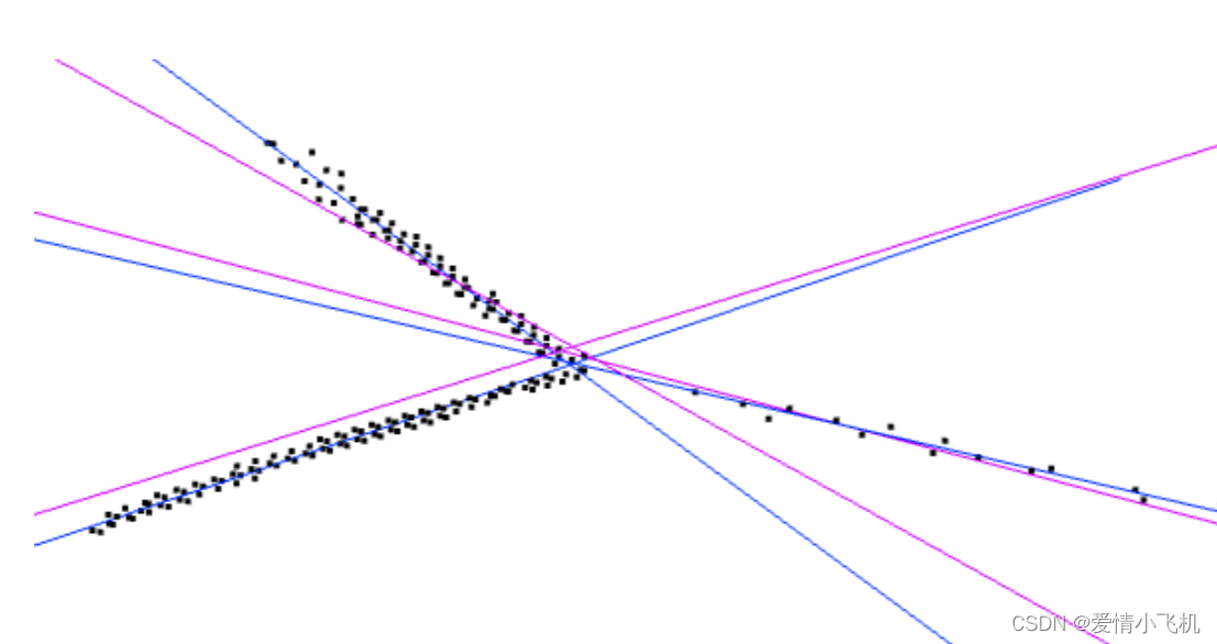
 此图中,粉色为LS,蓝色为OLS。可以看到由于去掉了一部分外点。OLS拟合直线的效果还是比较好的。

  • 1
    点赞
  • 7
    收藏
    觉得还不错? 一键收藏
  • 1
    评论

“相关推荐”对你有帮助么?

  • 非常没帮助
  • 没帮助
  • 一般
  • 有帮助
  • 非常有帮助
提交
评论 1
添加红包

请填写红包祝福语或标题

红包个数最小为10个

红包金额最低5元

当前余额3.43前往充值 >
需支付:10.00
成就一亿技术人!
领取后你会自动成为博主和红包主的粉丝 规则
hope_wisdom
发出的红包
实付
使用余额支付
点击重新获取
扫码支付
钱包余额 0

抵扣说明:

1.余额是钱包充值的虚拟货币,按照1:1的比例进行支付金额的抵扣。
2.余额无法直接购买下载,可以购买VIP、付费专栏及课程。

余额充值