paper reading：[第一代GCN] Spectral Networks and Deep Locally Connected Networks on Graphs

本文链接：https://blog.csdn.net/qq_41683065/article/details/104117593

这篇论文发表在 2014 ICLR 会议，是第一篇研究将CNN泛化到非欧式空间的论文，老师给我的时候注明了这是“第一代GCN” 。

主要贡献是将CNN泛化到非欧几里得空间，并提出两种并列的model，分别是基于spatial和基于spectral。

图卷积的一些知识：

黄色的文字为2020.02.24更新，主要是对图卷积的 spatial 方法有了新的理解，但是对于 spectral 方法还是抱有疑问，可能要去问问老师了。~~另外就是讲一些关于CNN和GCN的背景知识放到了后面。~~

参考了其他两位博主的论文笔记：

文章目录

two constructions of GCN

spatial construction：deep locally connected networks

局部连接的实现：

通过滤波器 $F$ 来实现。

滤波器的非0元素位置决定。由相应节点的neighborhoods决定，非0权重表示连接，为0的权重表示未连接。

下采样的实现：

下采样就是池化，在这里池化的方式为聚类

input all the feature maps over a cluster, and output a single feature for that cluster.

在这里插入图片描述

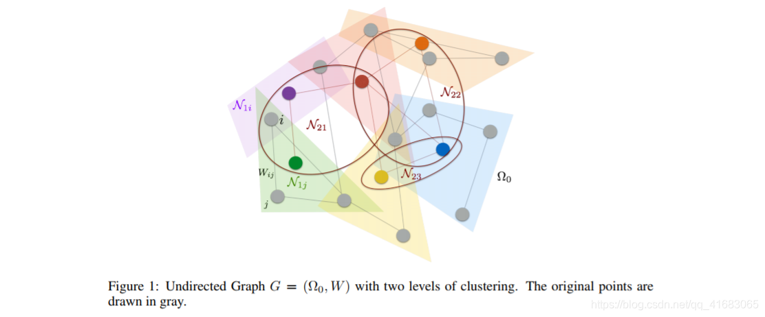
上图为聚类的示意图。

第一层为12个节点，第二次6个节点，第三次3个节点（图中未画出，用椭圆表示）。

深度局部连接的实现：

locally：neighborhoods
connected：每层与每层之间的神经元数目通过聚类而成。上一层的聚类结果对应下层的神经元。

各变量的含义：

Ω：各个层的输入信号。其中Ω₀是原始的输入信号。
K scales：网络的层数。
d_k clusters：第k层的下采样的cluster数，用于决定下一次输入feature的维度。
N_k,i：第k层的第i个neighborhoods，局部连接的接收域。（见figure 1）
f_k：第k层的滤波器数目，graph中每一个点的特征数。

在这里插入图片描述

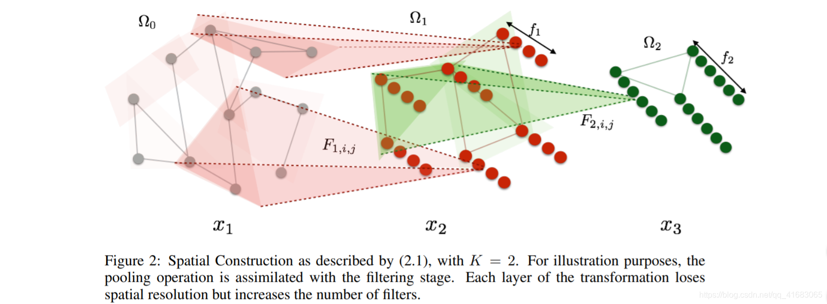
上图为卷积+池化的整个操作过程。

核心公式：

$x_{k+1,j}=L_k h (\sum_{i=1}^{f_{k-1}} F_{k,i,j} x_{k,i}) (j=1…f_k)$

对应的符号说明：

x_k,i ：第k层的信号的第i个特征。
F_k,i,j ：第k层的第j种滤波器的第i个值。F_k,i,j is a d_k−1 × d_k−1 sparse matrix with nonzero entries in the locations given by N_k。
h：非线性激活函数。
L_k ：第k层的池化操作。L_k outputs the result of a pooling operation over each cluster in Ω_k。

$(\sum_{i=1}^{f_{k-1}} F_{k,i,j} x_{k,i})$ 是对信号 $x_{k}$ 进行滤波器 $F_{k,j}$ 操作，局部性体现在滤波器中（滤波器由neighborhoods给定），表示其他的邻域内的信息向中心节点汇聚。之后经过 $h$ 的非线性激活和 $L_k$ 的池化（figure1 所示的聚类操作），得到下一层的信号。

每层的计算结果：

Each layer of the transformation loses spatial resolution but increases the number of filters.

即每层有两个结果（结合 Figure 2）：

loses spatial resolution：空间分辨率降低，即空间点数减少。
increases the number of filters：滤波器数目增加，即每个点特征数 $d_k$ 增。

那么对 spatial 方法来总结一下：

信号输入到model后，卷积操作通过与滤波器 $F$ 实现（ $F$ 由 neighborhoods 决定，实现 locally），之后通过聚类实现空间上的下采样，得到该层的输出结果。

模型评价：

优点：

it requires relatively weak regularity assumptions on the graph. Graphs having low intrinsic dimension have localized neighborhoods, even if no nice global embedding exists.

即：对于弱规则结构的graph依旧适用，且对于无良好global embedding的低维图也适用（原因是：低维图依旧存在 localized neighborhoods）。

缺点：

no easy way to induce weight sharing across different locations of the graph。

即：对于graph的不同位置，需采用不同的滤波器，从而导致==无法实现 weight sharing==权重共享。

CNN的单次卷积操作是由一个 filter 在整个数据立方（grid）上进行滑动（即 stride convolutions ），使得数据立方的不同位置可以使用同一个 fliter，而这个操作无法在 spatial construction 的 GCN 中实现。

spectral construction：spectrum of the graph Laplacian

原理

draws on the properties of convolutions in the Fourier domain.

In R^d , convolutions are linear operators diagonalised by the Fourier basis exp(iω·t), ω, t ∈ R^d.

One may then extend convolutions to general graphs by finding the corresponding “Fourier” basis.

This equivalence is given through the graph Laplacian, an operator which provides an harmonic analysis on the graphs.

即：卷积是被傅里叶基底对角化的线性操作子。

对这个概念进行推广，就是找到对graph而言的“傅里叶”基底，即 graph Laplacian。通过 graph Laplacian 得到 equivalence.

两种 Laplacian

combinatorial Laplacian

$L = D - W$

graph Laplacian

$L = I − D^{−1/2}W D^{−1/2}$

符号解释：

$D$ ：graph 的度矩阵 degree matric。
$W$ ：权重矩阵
$I$ ：对角矩阵

核心公式：

$x_{k+1,j}=h (V\sum_{i=1}^{f_{k-1}} F_{k,i,j}V^T x_{k,i}) (j=1…f_k)$

对应的符号说明：

$x_{k,i}$ ：第 k 层的信号的第 i 个特征。
$F_{k,i,j}$ ：第 k 层的第 **j **种滤波器的第 i 个值。 $F_{k,i,j}$ is a diagonal matrix.
$h$ ：实值非线性激活。
$V$ ：graph Laplacian $L$ 的特征向量，由特征值排序。the eigenvectors of the graph Laplacian $L$ , ordered by eigenvalue.

需要注意的是，此时 $F_{k,i,j}$ 并不能被 shared across locations，这要经由 smooth spectral multipliers 来实现。

公式解析：

graph Laplacian $L$ 的谱分解（或称为特征分解：将 $L$ 表示为特征值 $\lambda$ 和特征向量矩阵 $V$ 之积）可表示为
$\Lambda V^{-1} =V\Lambda V^{T}=V(\begin{pmatrix} \lambda_1& & \\ \ & \ddots& \\ & &\lambda_n\\ \end{pmatrix})V^{T}$
注意： $V^{-1}$ 可写为 $V^T$ 的条件为特征向量 eigenvectors 正交，此处满足条件。

graph 上的 Fourier 变换表示为
$X_{(N×1)} = V^T_{(N×N)} x_{(N×1)}$
对应 Fourier 逆变换为
$x_{(N×1)} = V_{(N×N)} X_{(N×1)}$
滤波器（卷积核）的 Fourier 变换为 $F$ ，即== $F$ 为定义在频谱上的滤波器，为对角矩阵==。

通过计算出 $L$ 的特征向量 $v$ 组成特征向量矩阵 $V$ ，利用矩阵 $V$ ，对权重进行对角化操作，来达到frenquency和smoothness的目的，并且可以将参数从 $m^2$ 个降到 $m$ 个。

整个卷积的原理就是卷积定理，求卷积的过程在频域上借一步而已：
$F(f(t)*g(t))=F(\omega)·G(\omega)$
综上所述： $V^T x_{k,i}$ 为对信号 $x_{k,i}$ 进行 Fourier 变换。 $\sum_{i=1}^{f_{k-1}} F_{k,i,j}V^T x_{k,i}$ 为频域上的信号和卷积核(滤波器)的卷积操作，通过 $V\sum_{i=1}^{f_{k-1}} F_{k,i,j}V^T x_{k,i}$ 中的 $V$ 再变回时域，从而完成时域的卷积操作。

需要注意的是，$V\sum_{i=1}^{f_{k-1}} F_{k,i,j}V^T $ 是线性操作子，非线性由 $h$ 引入。

另外，其他论文中的公式为
$(f*g)_G = U[ (U^T h) \odot (U^T f) ]$

smooth spectral：

Often, only the first $d$ eigenvectors of the Laplacian are useful in practice, which carry the smooth geometry of the graph. The cutoff frequency $d$ depends upon the intrinsic regularity of the graph and also the sample size. In that case, we can replace in (5) $V$ by $V_d$ , obtained by keeping the first $d$ columns of $V$ .

从信号的角度来看，信号的高频成份携带有信号的细节部分，去除其高频成份，即可实现 smooth。

实现 smooth 的方法就是仅仅保留特征向量矩阵 $V$ 中前 $d$ 个特征向量，原因是特征向量的排序是按照特征值的排序。

频域的对角操作子的好处和弊端：

好处：

将参数数目从 $O(n^2)$ 降低到 $O (n)$ .

弊端

most graphs have meaningful eigenvectors only for the very top of the spectrum.

Even when the individual high frequency eigenvectors are not meaningful, a cohort of high frequency eigenvectors may contain meaningful information.

However this construction may not be able to access this information because it is nearly diagonal at the highest frequencies.

简单来说，对于绝大多数 graph 而言，very top of the spectrum 的 eigenvectors 是意义的。而且高频特征向量的组合也含有信息。

而对角操作子只能同时提取单个特征向量的信息，即无法提取 a cohort of high frequency eigenvectors 所含有的信息。

translation invariant (平移不变性) 的实现：

linear operators $V F_{i,j}V^T$ in the Fourier basis ==> translation invariant ==> “classic” convolutions

spatial subsampling (空间下采样) 的实现：

spatial subsampling can also be obtained via dropping the last part of the spectrum of the Laplacian, leading to max-pooling, and ultimately to deep convolutonal networks。

局部连接和位置共享的实现：

in order to learn a layer in which features will be not only shared across locations but also well localized in the original domain, one can learn spectral multipliers which are smooth.

Smoothness can be prescribed by learning only a subsampled set of frequency multipliers and using an interpolation kernel to obtain the rest, such as cubic splines.

即：要实现每层的 feature 的位置共享和局部连接，spectral multipliers 应当 smooth，由对 frequency multipliers 的 subsample 来实现。

至此，GCN 在 spectral 上的卷积和池化的操作和局部连接和位置共享的实现已经介绍完毕，就可以实现deep convolutonal networks。

背景知识

CNN在image和audio recognition表现出色的原因：

ability to exploit the local translational invariance of signal classes over their domain 。

在各域上各类信号的“局部平移不变性”。比如对于语音信号的时移和图像中物体的平移，CNN的结果不变。

CNN的结构特点：

multiscale：这一点确实不知道该怎么理解。
hierarchical：层次化，信息的逐层提取。
local receptive fields：局部接收域（局部连接）。

由于gird的性质，使得CNN可以有以下的特点：

The translation structure(平移结构) ==> filters instead of generic linear maps(滤波器替代线性映射) ==> weight sharing(权重共享)
The metric on the grid ==> compactly supported filters ==> smaller than the size of the input signals(小尺寸滤波器)。
The multiscale dyadic clustering of the grid ==> stride convolutions and pooling(卷积和池化) ==> subsampling(下采样)

CNN的局限

Although the spatial convolutional structure can be exploited at several layers, typical CNN architectures do not assume any geometry in the “feature” dimension, resulting in 4-D tensors which are only convolutional along their spatial coordinates.

即对于一个4-D的tensor而言，其有X，Y，Z，feature四个维度，典型的CNN只能对X，Y，Z三个维度（即空间维度）进行卷积操作（通过3D convolution 操作），而不能对feature维度（特征维度）进行操作。