


此脚本读取用户指定网格点处的时间序列。它将Butterworth带通过滤器(bw_bandpass_filter)应用于该系列。原始(顶部)和过滤/信封(底部)系列说明了用法和结果。
;******************* ; bfband_1.ncl ; ; Concepts illustrated: ; - Specifying bandwidth ; - Applying 'bw_bandpass_filter' to time series at each grid point ; - plot raw time series ; - plot filterd and envelope series ;****************************** ;

# These libraries are automatically loaded from 6.2.0 onward # ;
load "$NCARG_ROOT/lib/ncarg/nclscripts/csm/gsn_code.ncl" ;
load "$NCARG_ROOT/lib/ncarg/nclscripts/csm/gsn_csm.ncl" ;
load "$NCARG_ROOT/lib/ncarg/nclscripts/csm/contributed.ncl" ;

***************************** ; Specify assorted constants ; ****************************

LAT = 0.0 ; specify single grid point
LON = 120.0
ca = 50                                        ; band width in days
cb = 40
pStrt = 19950101                               ; 4 years: winter 96-97 MJO gold standard
pLast = 19990101
pltType = "png"                                ; send graphics to PNG file
pltName = "bfband"

; ************************** ; Read the full time series for specified region ; This could easily be changed to just a temporal subset ; ************************************

diri = "./"
fili = "uwnd.day.850.anomalies.1980-2005.nc"
f = addfile(diri+fili, "r")
u = f->U_anom(:,{LAT},{LON})
printVarSummary(u)                             ; u(time)
dimu = dimsizes(u)
ntim = dimu(0)

; *********************************************** ; Butterworth filter ; . Return *both* the filtered and envelope time series ; ***********************************************

fca = 1.0/ca
fcb = 1.0/cb
dims = 0
opt = True
opt@return_envelope = True                     ; time series of filtered *and* envelope values
u_bf = bw_bandpass_filter (u,fca,fcb,opt,dims) ; (2,ntim)

; ********************************** ; Add meta data ; **********************************

copy_VarMeta(u, u_bf(0,:)) ; copy meta data: (2,time)
u_bf@long_name = "Band Pass: "+cb+"-"+ca+" day"
printVarSummary(u_bf) ; add time

; ************************************ ; Create new date array for use on the plot ; Select the start/end index (subscript) values ; *****************************************

date = cd_calendar(u_bf&time,-2)                 ; yyyymmdd
yrfrac = yyyymmdd_to_yyyyfrac (date, 0)
delete(yrfrac@long_name)
iStrt = ind(date.eq.pStrt)                       ; user specified dates
iLast = ind(date.eq.pLast)
delete(date)

; ********************* ; Create new date array for use on the plot ; *******************

plot = new ( 2, "graphic")
wks = gsn_open_wks (pltType,pltName)
res = True                                       ; plot mods desired
res@gsnDraw = False                              ; don't draw
res@gsnFrame = False                             ; don't advance frame yet
res@vpHeightF = 0.35                             ; change aspect ratio of plot
res@vpWidthF = 0.8
res@vpXF = 0.1                                   ; start plot at x ndc coord
res@gsnYRefLine = 0.0                            ; create a reference line
res@trYMinF =-4.0
res@trYMaxF = 4.0
res@tmXBFormat = "f"                             ;--- 1st plot
res@gsnCenterString = "Anomaly U ["+LAT+","+LON+"]"
plot(0) = gsn_csm_xy (wks,yrfrac(iStrt:iLast),u(iStrt:iLast),res)
                                                 ;--- 2nd plot
res@xyLineThicknesses = (/2.0,1.0/)
res@xyLineColors = (/"blue","red"/)              ; change line color
res@xyMonoDashPattern = True                     ; add a legend
res@pmLegendDisplayMode = "Always"               ; turn on legend
res@pmLegendSide = "Top"                         ; Change location of
res@pmLegendParallelPosF = .70                   ; move units right
res@pmLegendOrthogonalPosF = -0.5                ; more
neg = down
res@pmLegendWidthF = 0.10                        ; Change width and
res@pmLegendHeightF = 0.125                      ; height of legend.
res@lgLabelFontHeightF = .02                     ; change font height
res@lgPerimOn = False                            ; no box around
res@xyExplicitLegendLabels = (/"Filtered Data","Envelope"/)
res@gsnCenterString = "Butterworth Filtered: "+cb+"-"+ca+" day"
plot(1) = gsn_csm_xy (wks,yrfrac(iStrt:iLast),u_bf(:,iStrt:iLast),res)
resP = True
resP@gsnMaximize = True
gsn_panel(wks,plot,(/2,1/),resP) 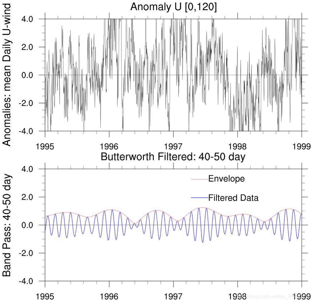


 1402
1402

 被折叠的 条评论
为什么被折叠?
被折叠的 条评论
为什么被折叠?
 到【灌水乐园】发言


