独立成分分析ICA/FastICA

最近在学习CSP，然后又注意到了ICA，这个算法之前就用过，但是没有系统的整理一下，所以就在这里梳理一下相关内容，方便以后查阅。

1 盲源分离（BlindSource Separation，BSS）的认识

1.1 盲源分离与ICA的关系

ICA 与盲源分离的方法具有非常密切的关系。ICA是实现盲源分离的其中一种，也是被最广泛使用的方法，故而，有必要在介绍ICA前，对盲源分离进行简要的介绍。

1.2 盲源分离的基础概念

盲源分离是由“鸡尾酒会问题”引出，该问题描述的是一场鸡尾酒会中有N个人一起说话，同时有N个录音设备，问怎样根据这N个录音文件恢复出N个人的原始语音，示意图如下。（ICA就是针对该问题所提出的一个算法。）

盲源分离： 根据源信号的统计特性，是指仅由观测的混合信号恢复（分离）出未知原始源信号的过程。通常观测到的混合信号来自多个传感器的输出，并且传感器的输出信号独立性（线性不相关）。

盲信号的“盲”字强调了两点：1)原始信号并不知道；2)对于信号混合的方法也不知道。

盲源分离的目的： 求得源信号的最佳估计。（当盲源分离的各分量相互独立时，就成为独立分量分析）。

1.3 盲源问题的原理性分析

寻找一个类似于【公式１】中矩阵$B$确定线性变换，使得随机变量$Y_i，i＝１,２，．．ｎ$尽可能独立，流程示意如下图所示：

因此，BSS的主要工作是寻找一个线性滤波器或者是一个权重矩阵$B$。理想的条件下，$B$矩阵是$A$矩阵的逆矩阵。由于参数空间不是欧几里得度量，在大多的情况下都是黎曼度量，因此对于$B$（或$W$）矩阵的求解选用自然梯度解法。

1.4 自然梯度求解法

2 独立成分分析（ICA）

2.1 形式化表达

其中随机向量$X=(x_1,x_2，\dots ，x_n)$表示观测数据或观测信号(observed data)，随机向量$S=(s_1，s_2，\dots ，s_n)$表示源信号，称为独立成分(independent components)，$A$称为$n\ast n$的混合矩阵(mixing matrix).
在该模型中，$X$表示的是一个随机向量，$x(t)$表示随机向量$X$的一个样本；$Y=BX=BAS$；$Y$是我们求解后的成分信号，$S$是源信号，若要使$Y$最大程度上逼近$S$，这实际上就是个优化过程，只需要满足解混合矩阵$B$是最佳估计$A$的逆矩阵就好。

上图所示是标准的独立成分分析模型，可以看作成一个生成模型(generativemodel)，它的意思是说观测信号是通过源信号混合而生成的，在这个意义下，独立成分也称为隐含或潜在交量(hidden／latent , nariable )，也就是说这些独立成分是无法直接观测到的，另一方面，混合系数矩阵$A$也是未知的。

这就是ICA的形式化表示，对于一个输入的$n$行$m$列矩阵，ICA的目标就是找到一个$n$行$n$列混淆矩阵$A$，使得变换后的矩阵仍为$n$行$m$列矩阵，但是每一行不再是多人说话的混合语音而是解混得到的某一个人的说话语音。

2.2 ICA模型的直观理解

为了进一步理解ICA的统计模型，我们假设两个独立分量服从下面的均匀分布：

选择均匀分布的取值范围，使得均值为0，方差为1。$S_{\mathrm{１}}$和$S_{\mathrm{２}}$的联合密度在正方形内是均匀的，这源于联合密度的基础定义：两个独立变量的联合密度是他们边密度的乘积。联合密度如下图所示，数据点是从分布中随机抽取。

现在混合这两个独立成分，我们取下面的混合矩阵：

这得出了两个混合变量，$X_1$和$X_2$，很容易得出混合数据在一个平行四边形上的均匀分布，如下图所示：

我们可以看到，随机变量$X_1$和$X_2$不再独立，换一种说法是，是否有可能从一个值去预测另一个值。假设$X_1$的值为最大或最小值，那么$X_2$的值就可以确定了。
如上图中红框圈起来的数据点所示。由此可知，$X_1$和$X_2$已经不再独立了。但是对于上上图中的随机变量$S_1$和$S_2$情况就不同了，如果我们知道$S_1$的值，那么无论通过什么方式都无法确定$S_2$的值。

估计ICA数据模型的问题现在成为仅利用混合$X_1$和$X_2$的信息来估计混合矩阵$A_0$，实际上，我们可以通过观察上图来直观的估计矩阵$A$：平行四边形的边的方向就是混合矩阵$A$的列所指的方向。这样独立成分分析的解可以通过确定混合方向来得到，但在标准的ICA中这样的计算是较为复杂的，我们可以寻找更为方便，计算简单，且适用于独 立成分的任何分布的算法，这里只给出ICA的直观解释。

2.3 算法步骤

其中第3步提到的白化预处理步骤如下图所示，白化也是一个值得深入学习的概念，是数据处理中一个常用的重要方法，这里有详细介绍：矩阵白化原理及推导。

2.4 MATLAB代码

function S = myICA(X)
%MYICM - The ICA(Independent Component Analysis) algorithm.
%   To seperate independent signals from a mixed matrix X, the unmixed
%   signals are saved as rows of matrix S.
%
%   S = myICA(X)
% 
%   Input - 
%   X: a N*M matrix with mixed signals containing M datas with N dimensions;
%   Output - 
%   S: a N*M matrix with unmixed signals.

%% ICA calculation
if ~ismatrix(X)             % 确定输入是否为矩阵
    error('Error!');
end

[n,m] = size(X);            % 取输入矩阵的维数
S = zeros(n,m);             % 构造一个空的输出矩阵，维度与输入一样
W_old = rand(n);            % 构造n*n的旋转矩阵W
for row = 1:n               % 初始的W可赋值为每行之和为1的随机矩阵
    W_old(row,:) = W_old(row,:)/sum(W_old(row,:));
end

delta = 0.001;              % 设置W更新的最小阈值
itera = 1000;               % 设置学习轮次
alfa = 0.01;                % 设置学习率
for T = 1:m                 % 对列循环
    for i = 1:itera         % 循环轮次
        weight = zeros(n,1);
        for line = 1:n
            weight(line) = 1-2*sigmoid(W_old(line,:)*X(:,T));
        end
        W_new = W_old+alfa*( (weight(line)*(X(:,T))')+ inv(W_old') );   % 更新W
        if sum(sum(abs(W_new-W_old))) <= delta   
            break;          % 如果W不再更新，则开始下一列的循环
        else
            W_old = W_new;
        end
    end
    S(:,T) = W_new*X(:,T);  % [n,m] = [n,n]*[n,m]
end

end

%% sigmoid function
%--------------------------------------------------------------------
function g = sigmoid(x)
    g = 1/(1+exp(-x));
end
%%

clear;close;clc;
%% ICA test
[s1,fs] = audioread('sound1.wav');
[s2,~] = audioread('sound2.wav');
s1 = s1(:)';
s2 = s2(:)';
s1 = s1/max(s1);
s2 = s2/max(s2);
L = min(length(s1),length(s2));
s1 = s1(1:L);
s2 = s2(1:L);

% 语音混叠
H = rand(5,2)*[s1;s2];
mx = mean(H,2);
H = H - mx*ones(1,L);   % subtract means from mixes 字段减去均值，中心化
X=H;
tic;
S = myICA(X(1:2,:));
toc
sound(X(1,:),fs);
sound(X(2,:),fs);
sound(S(1,:),fs);
sound(S(2,:),fs);

需要的音频：链接: https://pan.baidu.com/s/1b8dT6rz5-cr0r0DoyloXKw?pwd=yqe2 提取码: yqe2

3 算法改进：FastICA

3.1 形式化表达

事实上，ICA算法从提出至今就处于不断改进的进程中，到现在，经典的ICA算法已经基本不再使用，而是被一种名为FastICA的改进算法替代。顾名思义，该算法的优点在与Fast，即运算速度快。具体的改进点如下图所示。

3.2 MATLAB代码

function Y = myWhite(X,DIM)
%MYWHITE - The whitening function.
%   To calculate the white matex of input matrix X and 
%   the result after X being whitened. 
%   
%   Res = myWhite(X,DIM)
% 
%   Input - 
%   X: a N*M matrix containing M datas with N dimensions;
%   DIM: specifies a dimension DIM to arrange X.
%       DIM = 1: X(N*M)
%       DIM = 2: X(M*N)
%       DIM = otherwisw: error
%   Output - 
%   Y  : result matrix of X after being whitened;
%       Y.PCAW: PCA whiten result;
%       Y.ZCAW: ZCA whiten result.

%% parameter test
if nargin < 2
    DIM = 1;
end
if DIM == 2
    X = X';
elseif DIM~=1 && DIM~=2
    error('Error! Parameter DIM should be either 1 or 2.');
end
[~,M] = size(X);

%% whitening
% step1 PCA pre-processing
X = X - repmat(mean(X,2),1,M);        % de-mean
C = 1/M*X*(X');                       % calculate cov(X), or: C = cov((X)')
[eigrnvector,eigenvalue] = eig(C);    % calculate eigenvalue, eigrnvector
% TEST NOW: eigrnvector*(eigrnvector)' should be identity matrix.
% step2 PCA whitening
if all(diag(eigenvalue))    % no zero eigenvalue
    Xpcaw = eigenvalue^(-1/2) * (eigrnvector)' * X;
else
    vari = 1./sqrt(diag(eigenvalue)+1e-5);
    Xpcaw = diag(vari) * (eigrnvector)' * X;
end
% Xpczw = (eigenvalue+diag(ones(size(X,1),1)*(1e-5)))^(-1/2)*(eigrnvector)'*X;    % 数据正则化
% step3 ZCA whitening
Xzcaw = eigrnvector*Xpcaw;
% TEST NOW: cov((Xpczw)') and cov((Xzcaw)') should be identity matrix.

%% result output
Y.PCAW = Xpcaw;
Y.ZCAW = Xzcaw;

end

function Z = FastICA(X)
%FASTICA - The FastICA(Fast Independent Component Analysis) algorithm.
%   To seperate independent signals from a mixed matrix X, the unmixed
%   signals are saved as rows of matrix Z.
%
%   Z = FastICA(X)
% 
%   Input - 
%   X: a N*M matrix with mixed signals containing M datas with N dimensions;
%   Output - 
%   Z: a N*M matrix with unmixed signals.

%% 去均值
[M,T]=size(X);              % 获取输入矩阵的行列数，行数为观测数据的数目，列数为采样点数
average=mean((X'))';        % 均值
for i=1:M                   % 初始的W可赋值为每行之和为1的随机矩阵
    X(i,:)=X(i,:)-average(i)*ones(1,T);
end

%% 白化/球化
Y = myWhite(X,1);
Z = Y.PCAW;
% Z=X;
%% 迭代
Maxcount=10000;                 % 最大迭代次数
Critical=0.00001;               % 判断是否收敛
m=M;                            % 需要估计的分量的个数,输入矩阵的行数
W=rand(m);                      % 构造n*n的旋转矩阵W
for n=1:m                       % 按行去循环
    WP=W(:,n);                  % 初始权矢量（任意），取其中一列，[m, 1]
    %Y=WP'*Z;
    %G=Y.^3;%G为非线性函数，可取y^3等
    %GG=3*Y.^2；   %G的导数
    count=0;                    % 迭代次数
    LastWP=zeros(m,1);          % [m, 1]
    W(:,n)=W(:,n)/norm(W(:,n)); %单位化一列向量
    while (abs(WP-LastWP) & abs(WP+LastWP)) > Critical  %两个绝对值同时大于收敛条件
        count=count+1;          % 迭代次数
        LastWP=WP;              % 上次迭代的值
        %WP=1/T*Z*((LastWP'*Z).^3)'-3*LastWP;
        for i=1:m               % 按行去循环
            %更新
            WP(i)=mean( Z(i,:).*(tanh((LastWP)'*Z)) )-(mean(1-(tanh((LastWP))'*Z).^2)).*LastWP(i);
        end
        WPP=zeros(m,1);         % 施密特正交化，[m, 1]
        for j=1:n-1
            WPP=WPP+(WP'*W(:,j))*W(:,j);
        end
        WP=WP-WPP;
        WP=WP/(norm(WP));
        
        if count==Maxcount
            fprintf('未找到相应的信号');
            return;
        end
    end
    W(:,n)=WP;
end

%% 数据输出
Z=W'*Z;

end

clear;close;clc;
%% ICA test
[s1,fs] = audioread('sound1.wav');
[s2,~] = audioread('sound2.wav');
s1 = s1(:)';
s2 = s2(:)';
s1 = s1/max(s1);
s2 = s2/max(s2);
L = min(length(s1),length(s2));
s1 = s1(1:L);
s2 = s2(1:L);

% 语音混叠
H = rand(5,2)*[s1;s2];
mx = mean(H,2);
H = H - mx*ones(1,L);   % subtract means from mixes 字段减去均值，中心化
X=H;
tic;
S = FastICA(X(1:2,:));
toc
sound(X(1,:),fs);
sound(X(2,:),fs);
sound(S(1,:),fs);
sound(S(2,:),fs);

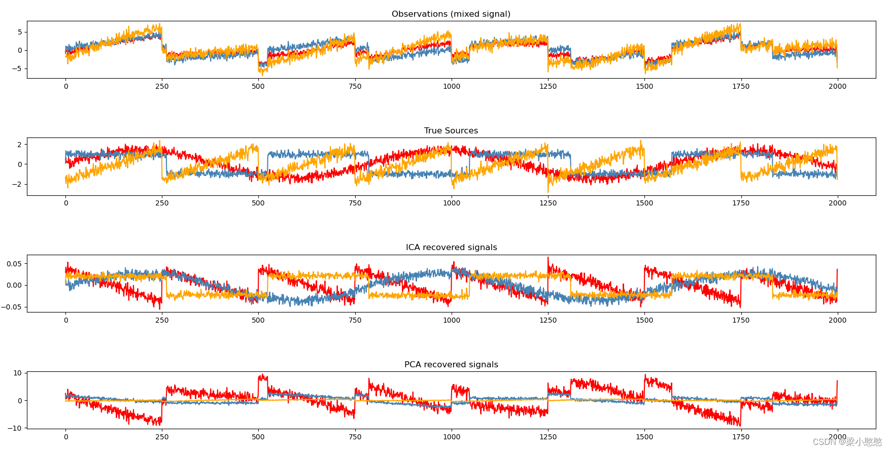
4 Python代码-sklearn

以下内容来自：Blind source separation using FastICA

import numpy as np
from scipy import signal
from sklearn.decomposition import FastICA, PCA
import matplotlib.pyplot as plt


################################### Generate sample data ###################################
np.random.seed(0)                           # 设置随机因子，让每次随机产生的数都一样
n_samples = 2000                            # 设置数据点的个数
time = np.linspace(0, 8, n_samples)         # 即从0到8闭区间，划分为n_samples个数据点

s1 = np.sin(2 * time)                       # Signal 1 : sinusoidal signal
s2 = np.sign(np.sin(3 * time))              # Signal 2 : square signal
s3 = signal.sawtooth(2 * np.pi * time)      # Signal 3: saw tooth signal

S = np.c_[s1, s2, s3]                       # 将s1, s2, s3组合起来，[2000. 3]
S += 0.2 * np.random.normal(size=S.shape)   # Add noise

S /= S.std(axis=0)                          # Standardize data,除标准差
# Mix data
A = np.array([[1, 1, 1], [0.5, 2, 1.0], [1.5, 1.0, 2.0]])  # Mixing matrix
X = np.dot(S, A.T)                          # Generate observations

################################### Fit ICA and PCA models ###################################
# Compute ICA
ica = FastICA(n_components=3)               # 设置ICA参数，components=3因为原始信号为三个
S_ = ica.fit_transform(X)                   # Reconstruct signals，重建信号
A_ = ica.mixing_                            # Get estimated mixing matrix，得到估计的混合矩阵

# We can `prove` that the ICA model applies by reverting the unmixing.
assert np.allclose(X, np.dot(S_, A_.T) + ica.mean_) # 如果两个数组在给定的公差范围内相等，则返回True；否则，返回True。assert：测试条件是否返回 True：

# For comparison, compute PCA
pca = PCA(n_components=3)
H = pca.fit_transform(X)                    # Reconstruct signals based on orthogonal components

################################### Plot results ###################################
plt.figure()

models = [X, S, S_, H]
names = [
    "Observations (mixed signal)",
    "True Sources",
    "ICA recovered signals",
    "PCA recovered signals",
]
colors = ["red", "steelblue", "orange"]

for ii, (model, name) in enumerate(zip(models, names), 1): # 将元组转换为可枚举对象，定义枚举对象的起始编号为1，默认值为 0。zip：把两个元组连接起来
    plt.subplot(4, 1, ii)
    plt.title(name)
    for sig, color in zip(model.T, colors):
        plt.plot(sig, color=color)

plt.tight_layout()
plt.show()

5 Python代码-MNE

以下内容来自：Repairing artifacts with ICA

import os
import mne
from mne.preprocessing import (ICA, create_eog_epochs, create_ecg_epochs,corrmap)
import matplotlib.pyplot as plt


################################################################### Load data ###################################################################
sample_data_folder = mne.datasets.sample.data_path()
sample_data_raw_file = os.path.join(sample_data_folder, 'MEG', 'sample',
                                    'sample_audvis_filt-0-40_raw.fif')
raw = mne.io.read_raw_fif(sample_data_raw_file)
# Here we'll crop to 60 seconds and drop gradiometer channels for speed
raw.crop(tmax=60.).pick_types(meg='mag', eeg=True, stim=True, eog=True)
raw.load_data()

################################################################### Visualizing the artifacts ###################################################################
# pick some channels that clearly show heartbeats and blinks
# regexp = r'(MEG [12][45][123]1|EEG 00.)'
# artifact_picks = mne.pick_channels_regexp(raw.ch_names, regexp=regexp)
# raw.plot(order=artifact_picks, n_channels=len(artifact_picks),
#          show_scrollbars=False)

# eog_evoked = create_eog_epochs(raw).average()
# eog_evoked.apply_baseline(baseline=(None, -0.2))
# eog_evoked.plot_joint()

# ecg_evoked = create_ecg_epochs(raw).average()
# ecg_evoked.apply_baseline(baseline=(None, -0.2))
# ecg_evoked.plot_joint()

################################################################### Filtering to remove slow drifts ###################################################################
filt_raw = raw.copy().filter(l_freq=1., h_freq=None)

################################################################### Fitting and plotting the ICA solution ###################################################################
# ica = ICA(n_components=15, max_iter='auto', random_state=97)
# ica.fit(filt_raw)

# raw.load_data()
# ica.plot_sources(raw, show_scrollbars=False)

# ica.plot_components()

# # blinks
# ica.plot_overlay(raw, exclude=[0], picks='eeg')
# # heartbeats
# ica.plot_overlay(raw, exclude=[1], picks='mag')

# ica.plot_properties(raw, picks=[0, 1])

################################################################### Selecting ICA components manually ###################################################################
# ica.exclude = [0, 1]  # indices chosen based on various plots above

# # ica.apply() changes the Raw object in-place, so let's make a copy first:
# reconst_raw = raw.copy()
# ica.apply(reconst_raw)

# raw.plot(order=artifact_picks, n_channels=len(artifact_picks),
#          show_scrollbars=False)
# reconst_raw.plot(order=artifact_picks, n_channels=len(artifact_picks),
#                  show_scrollbars=False)
# plt.show()
# del reconst_raw

################################################################### Using an EOG channel to select ICA components ###################################################################
# ica.exclude = []
# # find which ICs match the EOG pattern
# eog_indices, eog_scores = ica.find_bads_eog(raw)
# ica.exclude = eog_indices

# # barplot of ICA component "EOG match" scores
# ica.plot_scores(eog_scores)

# # plot diagnostics
# ica.plot_properties(raw, picks=eog_indices)

# # plot ICs applied to raw data, with EOG matches highlighted
# ica.plot_sources(raw, show_scrollbars=False)

# # plot ICs applied to the averaged EOG epochs, with EOG matches highlighted
# ica.plot_sources(eog_evoked)

################################################################### Using a simulated channel to select ICA components ###################################################################
# ica.exclude = []
# # find which ICs match the ECG pattern
# ecg_indices, ecg_scores = ica.find_bads_ecg(raw, method='correlation',
#                                             threshold='auto')
# ica.exclude = ecg_indices

# # barplot of ICA component "ECG match" scores
# ica.plot_scores(ecg_scores)

# # plot diagnostics
# ica.plot_properties(raw, picks=ecg_indices)

# # plot ICs applied to raw data, with ECG matches highlighted
# ica.plot_sources(raw, show_scrollbars=False)

# # plot ICs applied to the averaged ECG epochs, with ECG matches highlighted
# ica.plot_sources(ecg_evoked)


# # refit the ICA with 30 components this time
# new_ica = ICA(n_components=30, max_iter='auto', random_state=97)
# new_ica.fit(filt_raw)

# # find which ICs match the ECG pattern
# ecg_indices, ecg_scores = new_ica.find_bads_ecg(raw, method='correlation',
#                                                 threshold='auto')
# new_ica.exclude = ecg_indices

# # barplot of ICA component "ECG match" scores
# new_ica.plot_scores(ecg_scores)

# # plot diagnostics
# new_ica.plot_properties(raw, picks=ecg_indices)

# # plot ICs applied to raw data, with ECG matches highlighted
# new_ica.plot_sources(raw, show_scrollbars=False)

# # plot ICs applied to the averaged ECG epochs, with ECG matches highlighted
# new_ica.plot_sources(ecg_evoked)

# # clean up memory before moving on
# del raw, ica, new_ica


################################################################### Selecting ICA components using template matching ###################################################################
# raws = list()
# icas = list()

# for subj in range(4):
#     # EEGBCI subjects are 1-indexed; run 3 is a left/right hand movement task
#     fname = mne.datasets.eegbci.load_data(subj + 1, runs=[3])[0]
#     raw = mne.io.read_raw_edf(fname).load_data().resample(50)
#     # remove trailing `.` from channel names so we can set montage
#     mne.datasets.eegbci.standardize(raw)
#     raw.set_montage('standard_1005')
#     # high-pass filter
#     raw_filt = raw.copy().load_data().filter(l_freq=1., h_freq=None)
#     # fit ICA, using low max_iter for speed
#     ica = ICA(n_components=30, max_iter=100, random_state=97)
#     ica.fit(raw_filt, verbose='error')
#     raws.append(raw)
#     icas.append(ica)

# use the first subject as template; use Fpz as proxy for EOG
# raw = raws[0]
# ica = icas[0]
# eog_inds, eog_scores = ica.find_bads_eog(raw, ch_name='Fpz')
# corrmap(icas, template=(0, eog_inds[0]))

# for index, (ica, raw) in enumerate(zip(icas, raws)):
#     with mne.viz.use_browser_backend('matplotlib'):
#         fig = ica.plot_sources(raw, show_scrollbars=False)
#     fig.subplots_adjust(top=0.9)  # make space for title
#     fig.suptitle('Subject {}'.format(index))
# plt.show()

# corrmap(icas, template=(0, eog_inds[0]), threshold=0.9)

# corrmap(icas, template=(0, eog_inds[0]), threshold=0.9, label='blink',
#         plot=False)
# print([ica.labels_ for ica in icas])

# icas[3].plot_components(picks=icas[3].labels_['blink'])
# icas[3].exclude = icas[3].labels_['blink']
# icas[3].plot_sources(raws[3], show_scrollbars=False)
# plt.show()

# template_eog_component = icas[0].get_components()[:, eog_inds[0]]
# corrmap(icas, template=template_eog_component, threshold=0.9)
# print(template_eog_component)

################################################################### Compute ICA components on Epochs ###################################################################
filt_raw.pick_types(meg=True, eeg=False, exclude='bads', stim=True).load_data()
filt_raw.filter(1, 30, fir_design='firwin')

# peak-to-peak amplitude rejection parameters
reject = dict(mag=4e-12)
# create longer and more epochs for more artifact exposure
events = mne.find_events(filt_raw, stim_channel='STI 014')
# don't baseline correct epochs
epochs = mne.Epochs(filt_raw, events, event_id=None, tmin=-0.2, tmax=0.5,
                    reject=reject, baseline=None)

ica = ICA(n_components=15, method='fastica', max_iter="auto").fit(epochs)

ecg_epochs = create_ecg_epochs(filt_raw, tmin=-.5, tmax=.5)
ecg_inds, scores = ica.find_bads_ecg(ecg_epochs, threshold='auto')

# ica.plot_components(ecg_inds)

# ica.plot_properties(epochs, picks=ecg_inds)

ica.plot_sources(filt_raw, picks=ecg_inds, show_scrollbars=False)
plt.show()

参考文章

基于FastICA的声源分离实例（matlab代码）

独立成分分析FastICA算法原理

学习笔记 | 独立成分分析(ICA, FastICA)及应用

Blind source separation using FastICA

Repairing artifacts with ICA