线性回归模型

一元线性回归模型的介绍与应用

一元线性回归模型

回归方程形式：，i=1,2,...n,其中需满足以下四个假设条件

a.正态性假设，即是服从正态分布的随机变量

b.无偏性假设，即E()=0

c.同方差性假设，即所有的方差都相同；同时也说明了与自变量，因变量之间都是相互独立的

d.独立性假设，之间相互独立，且满足COV(,)=0(ij)

根据误差平方和最小的原则，用最小二乘法求解参数a,b：

 

一元回归模型python的实现：

import pandas as pd
import statsmodels.api as sm
income = pd.read_csv(r'D:\download\python数据分析与挖掘\第11章 线性回归模型\Salary_Data.csv')
# 构建回归模型
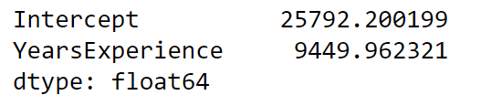
fit = sm.formula.ols('Salary~YearsExperience',data = income).fit()
fit.params  # 返回参数


'''
sm.ols(formula, data, subset=None, drop_cols=None)

formula：以字符串的形式指定线性回归模型的公式，如'y~x'就表示简单线性回归模型
data：指定建模的数据集
subset：通过bool类型的数组对象，获取data的子集用于建模
drop_cols：指定需要从data中删除的变量
'''

数据集：

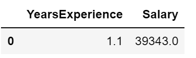
结果：

查看两变量相关性：

income.Salary.corr(income.YearsExperience) #0.98

多元线性回归模型的系数推导

多元回归模型的定义

 

多元回归模型python的实现：

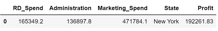
数据集：

查看相关性

profit.drop('State',axis=1).corrwith(profit.Profit) # Profit变量与其他三个连续变量的相关性

 

profit.drop('State',axis=1).corr() # 四个连续变量两两之间的相关性

 

from sklearn import model_selection
profit = pd.read_excel(r'D:\download\python数据分析与挖掘\第11章 线性回归模型\Predict to Profit.xlsx')
# profit.head(1)

# 将数据拆分为训练集和测试集
train,test = model_selection.train_test_split(profit,test_size = 0.2,random_state=1234)
# 根据train数据建模
model = sm.formula.ols('Profit~RD_Spend+Administration+Marketing_Spend+C(State)',data=train).fit() # State加C()表示分类变量,State有三个类别
print("模型的偏回归系数分别为：\n",model.params)

# 删除test数据集中的Profit变量，用剩下的自变量进行预测
test_X = test.drop(labels='Profit',axis=1)
pred=model.predict(exog=test_X)
print("对比预测值和实际值的差异：\n",pd.DataFrame({'Prediction':pred,'Real':test.Profit}))

结果如下，state默认将离散变量State的California作为对照组（共生性）。下面另一段代码是手动为State设置哑变量，并砍掉New York做的预测结果

# 生成哑变量
dummies = pd.get_dummies(profit.State)
# 新增哑变量列，生成新数据
profit_new = pd.concat([profit,dummies],axis=1)
# 删除State变量和California变量（因为State变量已被分解为哑变量，New York变量需要作为参照组）
profit_new.drop(labels = ['State','New York'],axis = 1,inplace = True)
train,test=model_selection.train_test_split(profit_new,test_size=0.2,random_state=1234)
model = sm.formula.ols('Profit~RD_Spend+Administration+Marketing_Spend+Florida+California',data = train).fit()
print('模型的偏回归系数分别为：\n',model.params)

 

线性回归模型的假设检验

模型的F检验

1. 提出问题的原假设和备择假设
2. 在原假设的条件下，构造统计量F
3. 根据样本信息，计算统计量的值
4. 对比统计量的值和理论F分布的值，当统计量值超过理论值时，拒绝原假设，否则接受原假设

# 模型的F检验

# 1.计算F统计量
import numpy as np
# 计算建模数据中因变量的均值
ybar = train.Profit.mean()
# 统计模型model中变量个数以及训练集观测个数
p = model.df_model
n = train.shape[0]
# 计算回归平方和
RSS = np.sum((model.fittedvalues-ybar)**2)
# 计算残差平方和
ESS = np.sum(model.resid**2)
# 计算F统计量
F = (RSS/p)/(ESS/(n-p-1))
print(F,"直接得到F：",model.fvalue) #174.63721716844725 174.6372171570355

# 2. 与F分布的理论值对比
# 导入模块
from scipy.stats import f
# 计算F分布的理论值
F_Theroy = f.ppf(q=0.95, dfn = p,dfd = n-p-1)
print('F分布的理论值为：',F_Theroy) # F分布的理论值为： 2.502635007415366

结论：

计算出来的F统计量值174.64远远大于F分布的理论值2.50，所以应当拒绝原假设，即认为多元线性回归模型是显著的，也就是说回归模型的偏回归系数都不全为0

参数的T检验

查看模型的概览信息

从结果可以看出，只有截距项Intercept和研发成本RD_Spend通过了显著性检验，其P值远小于0.05

model.summary()

OLS Regression Results

Dep. Variable:	Profit	R-squared:	0.964
Model:	OLS	Adj. R-squared:	0.958
Method:	Least Squares	F-statistic:	174.6
Date:	Thu, 22 Apr 2021	Prob (F-statistic):	9.74e-23
Time:	23:34:37	Log-Likelihood:	-401.20
No. Observations:	39	AIC:	814.4
Df Residuals:	33	BIC:	824.4
Df Model:	5
Covariance Type:	nonrobust

	coef	std err	t	P>|t|	[0.025	0.975]
Intercept	5.807e+04	6846.305	8.482	0.000	4.41e+04	7.2e+04
RD_Spend	0.8035	0.040	19.988	0.000	0.722	0.885
Administration	-0.0578	0.051	-1.133	0.265	-0.162	0.046
Marketing_Spend	0.0138	0.015	0.930	0.359	-0.016	0.044
Florida	1440.8627	3059.931	0.471	0.641	-4784.615	7666.340
California	513.4683	3043.160	0.169	0.867	-5677.887	6704.824

Omnibus:	1.721	Durbin-Watson:	1.896
Prob(Omnibus):	0.423	Jarque-Bera (JB):	1.148
Skew:	0.096	Prob(JB):	0.563
Kurtosis:	2.182	Cond. No.	1.60e+06

Warnings:
[1] Standard Errors assume that the covariance matrix of the errors is correctly specified.
[2] The condition number is large, 1.6e+06. This might indicate that there are
strong multicollinearity or other numerical problems.