


 本文详细介绍qiime2R包的使用方法,包括如何将qiime2中的特征表、分类文件及进化树文件导入R软件,进行图形绘制及统计分析。文章通过Movingpictures教程数据,演示了读取qza文件、构建Phyloseq对象、计算α多样性、绘制PCoA图、制作热图和柱状图等操作,并展示了如何进行差异性丰度计算和绘制造型树。
qiime2R包讲qiime2中的最终特征表文件(table.qza),分类文件(taxonomy.qza)及进化树文件直接导入R软件中,进行图形的绘制及统计分析。
功能如下:
read_qza()- Function for reading artifacts (.qza).qza_to_phyloseq()- Imports multiple artifacts to produce a phyloseq object.read_q2metadata()- Reads qiime2 metadata file (containing q2-types definition line)write_q2manifest()- Writes a read manifest file to import data into qiime2theme_q2r()- A ggplot2 theme for publication-type figures.print_provenance()- A function to display provenance information.is_q2metadata()- A function to check if a file is a qiime2 metadata file.parse_taxonomy()- A function to parse taxonomy strings and return a table where each column is a taxonomic class.parse_ordination()- A function to parse the internal ordination format.read_q2biom- A function for reading QIIME2 biom files in format v2.1make_clr- Transform feature table using centered log2 ratio.make_proportion- Transform feature table to proportion (sum to 1).make_percent- Transform feature to percent (sum to 100).interactive_table- Create an interactive table in Rstudio viewer or rmarkdown html.summarize_taxa- Create a list of tables with abundances sumed to each taxonomic level.taxa_barplot- Create a stacked barplot using ggplot2.taxa_heatmap- Create a heatmap of taxonomic abundances using gplot2
qiime2R包的安装
if (!requireNamespace("devtools", quietly = TRUE)){install.packages("devtools")}
devtools::install_github("jbisanz/qiime2R")
读取qza文件(这里以Moving pictures tutorial数据为例)
https://docs.qiime2.org/2020.8/tutorials/moving-pictures/
SVs<-read_qza("table.qza")
names(SVs)
[1] "uuid"       "type"       "format"     "contents"   "version"
[6] "data"       "provenance"

SVs$data[1:5,1:5] #show first 5 samples and first 5 taxa

SVs$uuid
[1] "706b6bce-8f19-4ae9-b8f5-21b14a814a1b"

SVs$type
[1] "FeatureTable[Frequency]"
读取metadata
metadata<-read_q2metadata("sample-metadata.tsv")
head(metadata) # show top lines of metadata
#  SampleID barcode-sequence body-site year month day   subject reported-antibiotic-usage days-since-experiment-start
#2     L1S8     AGCTGACTAGTC       gut 2008    10  28 subject-1                       Yes                           0
#3    L1S57     ACACACTATGGC       gut 2009     1  20 subject-1                        No                          84
#4    L1S76     ACTACGTGTGGT       gut 2009     2  17 subject-1                        No                         112
#5   L1S105     AGTGCGATGCGT       gut 2009     3  17 subject-1                        No                         140
#6   L2S155     ACGATGCGACCA left palm 2009     1  20 subject-1                        No                          84
#7   L2S175     AGCTATCCACGA left palm 2009     2  17 subject-1
读取taxonomy
taxonomy<-read_qza("taxonomy.qza")
head(taxonomy$data)
#                        Feature.ID                                                                                                                            Taxon Confidence
#1 4b5eeb300368260019c1fbc7a3c718fc                          k__Bacteria; p__Bacteroidetes; c__Bacteroidia; o__Bacteroidales; f__Bacteroidaceae; g__Bacteroides; s__  0.9972511
#2 fe30ff0f71a38a39cf1717ec2be3a2fc                           k__Bacteria; p__Proteobacteria; c__Betaproteobacteria; o__Neisseriales; f__Neisseriaceae; g__Neisseria  0.9799427
#3 d29fe3c70564fc0f69f2c03e0d1e5561                                k__Bacteria; p__Firmicutes; c__Bacilli; o__Lactobacillales; f__Streptococcaceae; g__Streptococcus  1.0000000
#4 868528ca947bc57b69ffdf83e6b73bae                          k__Bacteria; p__Bacteroidetes; c__Bacteroidia; o__Bacteroidales; f__Bacteroidaceae; g__Bacteroides; s__  0.9955859
#5 154709e160e8cada6bfb21115acc80f5                               k__Bacteria; p__Bacteroidetes; c__Bacteroidia; o__Bacteroidales; f__Bacteroidaceae; g__Bacteroides  1.0000000
#6 1d2e5f3444ca750c85302ceee2473331 k__Bacteria; p__Proteobacteria; c__Gammaproteobacteria; o__Pasteurellales; f__Pasteurellaceae; g__Haemophilus; s__parainfluenzae  0.9455365
taxonomy<-parse_taxonomy(taxonomy$data)
head(taxonomy)
#                                  Kingdom         Phylum               Class           Order           Family         Genus        Species
#4b5eeb300368260019c1fbc7a3c718fc Bacteria  Bacteroidetes         Bacteroidia   Bacteroidales   Bacteroidaceae   Bacteroides           <NA>
#fe30ff0f71a38a39cf1717ec2be3a2fc Bacteria Proteobacteria  Betaproteobacteria    Neisseriales    Neisseriaceae     Neisseria           <NA>
#d29fe3c70564fc0f69f2c03e0d1e5561 Bacteria     Firmicutes             Bacilli Lactobacillales Streptococcaceae Streptococcus           <NA>
#868528ca947bc57b69ffdf83e6b73bae Bacteria  Bacteroidetes         Bacteroidia   Bacteroidales   Bacteroidaceae   Bacteroides           <NA>
#154709e160e8cada6bfb21115acc80f5 Bacteria  Bacteroidetes         Bacteroidia   Bacteroidales   Bacteroidaceae   Bacteroides           <NA>
#1d2e5f3444ca750c85302ceee2473331 Bacteria Proteobacteria Gammaproteobacteria  Pasteurellales  Pasteurellaceae   Haemophilus parainfluenzae
构建 Phyloseq
physeq<-qza_to_phyloseq(
    features="inst/artifacts/2020.2_moving-pictures/table.qza",
    tree="inst/artifacts/2020.2_moving-pictures/rooted-tree.qza",
    taxonomy="inst/artifacts/2020.2_moving-pictures/taxonomy.qza",
    metadata = "inst/artifacts/2020.2_moving-pictures/sample-metadata.tsv"
    )
physeq
## phyloseq-class experiment-level object
## otu_table()   OTU Table:         [ 759 taxa and 34 samples ]
## sample_data() Sample Data:       [ 34 samples by 10 sample variables ]
## tax_table()   Taxonomy Table:    [ 759 taxa by 7 taxonomic ranks ]
## phy_tree()    Phylogenetic Tree: [ 759 tips and 757 internal nodes ]
结果展示
Alpha diversity
library(tidyverse)
library(qiime2R)

metadata<-read_q2metadata("sample-metadata.tsv")
shannon<-read_qza("shannon_vector.qza")

shannon<-shannon$data %>% rownames_to_column("SampleID") # this moves the sample names to a new column that matches the metadata and allows them to be merged

gplots::venn(list(metadata=metadata$SampleID, shannon=shannon$SampleID))
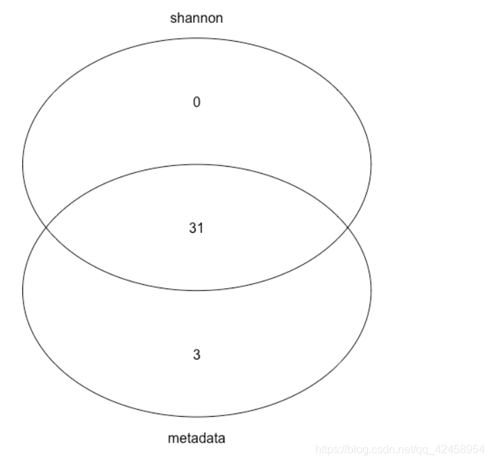
其中有3个样本无shannon值,接下来将进一步探索该三个样本
metadata<-
metadata %>%
left_join(shannon)
head(metadata)
# SampleID barcode-sequence body-site year month day subject reported-antibiotic-usage days-since-experiment-start shannon
#1 L1S8 AGCTGACTAGTC gut 2008 10 28 subject-1 Yes 0 3.188316
#2 L1S57 ACACACTATGGC gut 2009 1 20 subject-1 No 84 3.985702
#3 L1S76 ACTACGTGTGGT gut 2009 2 17 subject-1 No 112 3.461625
#4 L1S105 AGTGCGATGCGT gut 2009 3 17 subject-1 No 140 3.972339
#5 L2S155 ACGATGCGACCA left palm 2009 1 20 subject-1 No 84 5.064577
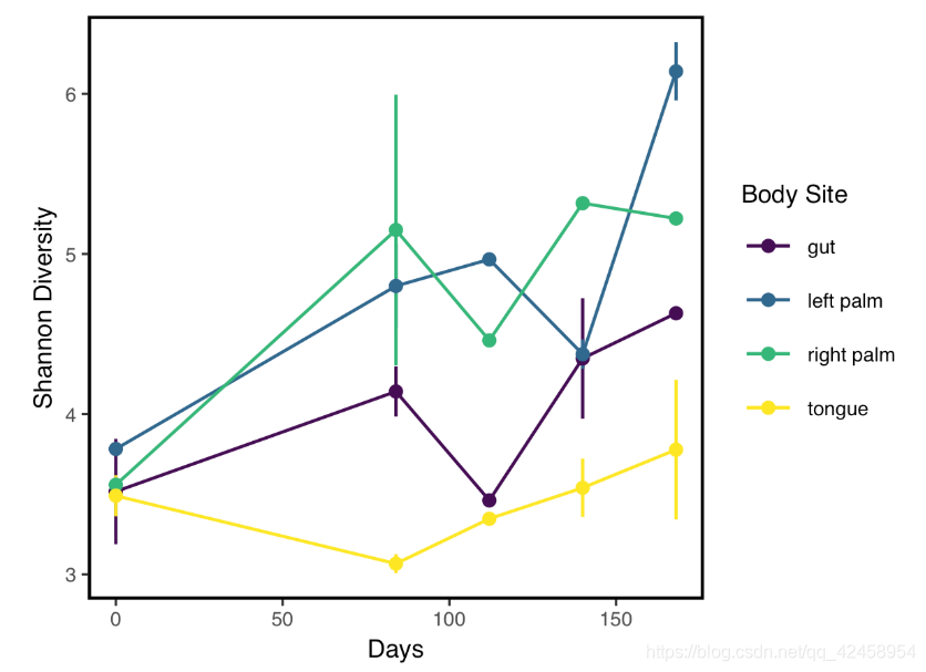
#6 L2S175 AGCTATCCACGA left palm 2009 2 17 subject-1 metadata %>%
filter(!is.na(shannon)) %>%
ggplot(aes(x=`days-since-experiment-start`, y=shannon, color=`body-site`)) +
stat_summary(geom="errorbar", fun.data=mean_se, width=0) +
stat_summary(geom="line", fun.data=mean_se) +
stat_summary(geom="point", fun.data=mean_se) +
xlab("Days") +
ylab("Shannon Diversity") +
theme_q2r() + # try other themes like theme_bw() or theme_classic()
scale_color_viridis_d(name="Body Site") # use different color scale which is color blind friendly
ggsave("Shannon_by_time.pdf", height=3, width=4, device="pdf") # save a PDF 3 inches by 4 inches
抗生素使用对多样性的影响
metadata %>%
  filter(!is.na(shannon)) %>%
  ggplot(aes(x=`reported-antibiotic-usage`, y=shannon, fill=`reported-antibiotic-usage`)) +
  stat_summary(geom="bar", fun.data=mean_se, color="black") + #here black is the outline for the bars
  geom_jitter(shape=21, width=0.2, height=0) +
  coord_cartesian(ylim=c(2,7)) + # adjust y-axis
  facet_grid(~`body-site`) + # create a panel for each body site
  xlab("Antibiotic Usage") +
  ylab("Shannon Diversity") +
  theme_q2r() +
  scale_fill_manual(values=c("cornflowerblue","indianred")) + #specify custom colors
  theme(legend.position="none") #remove the legend as it isn't needed
  ggsave("../../../images/Shannon_by_abx.pdf", height=3, width=4, device="pdf") # save a PDF 3 inches by 4 inches
其中两个样本间多样性的比较
metadata %>%
  filter(!is.na(shannon)) %>%
  ggplot(aes(x=subject, y=shannon, fill=`subject`)) +
  stat_summary(geom="bar", fun.data=mean_se, color="black") + #here black is the outline for the bars
  geom_jitter(shape=21, width=0.2, height=0) +
  coord_cartesian(ylim=c(2,7)) + # adjust y-axis
  facet_grid(~`body-site`) + # create a panel for each body site
  xlab("Antibiotic Usage") +
  ylab("Shannon Diversity") +
  theme_q2r() +
  scale_fill_manual(values=c("cornflowerblue","indianred")) + #specify custom colors
  theme(legend.position="none") #remove the legend as it isn't needed
  ggsave("Shannon_by_person.pdf", height=3, width=4, device="pdf") # save a PDF 3 inches by 4 inches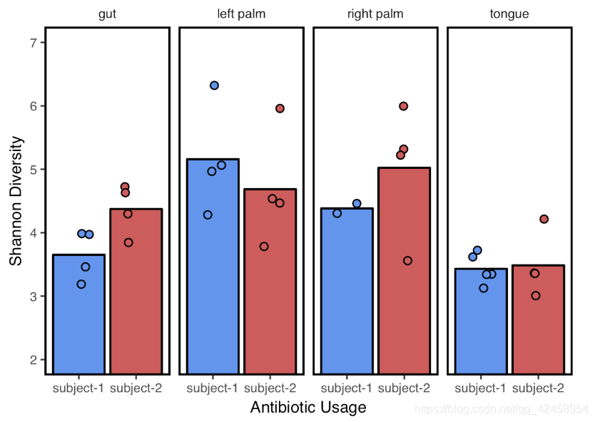
PCoA图的绘制
library(tidyverse)
library(qiime2R)

metadata<-read_q2metadata("sample-metadata.tsv")
uwunifrac<-read_qza("unweighted_unifrac_pcoa_results.qza")
shannon<-read_qza("shannon_vector.qza")$data %>% rownames_to_column("SampleID")

uwunifrac$data$Vectors %>%
  select(SampleID, PC1, PC2) %>%
  left_join(metadata) %>%
  left_join(shannon) %>%
  ggplot(aes(x=PC1, y=PC2, color=`body-site`, shape=`reported-antibiotic-usage`, size=shannon)) +
  geom_point(alpha=0.5) + #alpha controls transparency and helps when points are overlapping
  theme_q2r() +
  scale_shape_manual(values=c(16,1), name="Antibiotic Usage") + #see http://www.sthda.com/sthda/RDoc/figure/graphs/r-plot-pch-symbols-points-in-r.png for numeric shape codes
  scale_size_continuous(name="Shannon Diversity") +
  scale_color_discrete(name="Body Site")
ggsave("PCoA.pdf", height=4, width=5, device="pdf") # save a PDF 3 inches by 4 inches 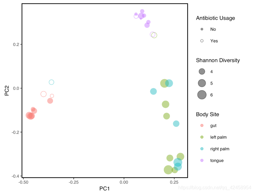
Heatmap
library(tidyverse)
library(qiime2R)

metadata<-read_q2metadata("sample-metadata.tsv")
SVs<-read_qza("table.qza")$data
taxonomy<-read_qza("taxonomy.qza")$data %>% parse_taxonomy()

taxasums<-summarize_taxa(SVs, taxonomy)$Genus

taxa_heatmap(taxasums, metadata, "body-site")

ggsave("heatmap.pdf", height=4, width=8, device="pdf") # save a PDF 4 inches by 8 inches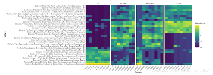
物种分类柱状图的绘制
library(tidyverse)
library(qiime2R)

metadata<-read_q2metadata("sample-metadata.tsv")
SVs<-read_qza("table.qza")$data
taxonomy<-read_qza("taxonomy.qza")$data %>% parse_taxonomy()

taxasums<-summarize_taxa(SVs, taxonomy)$Genus

taxa_barplot(taxasums, metadata, "body-site")

ggsave("barplot.pdf", height=4, width=8, device="pdf") # save a PDF 4 inches by 8 inches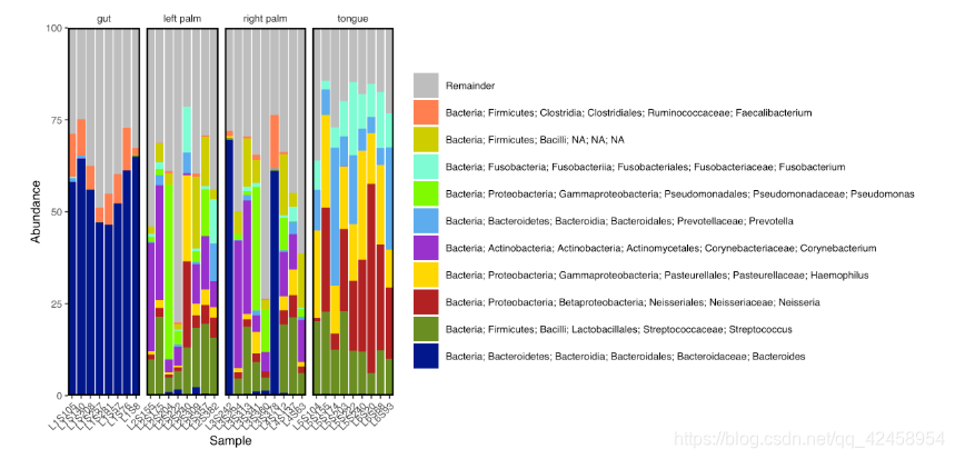
差异性丰度计算
library(tidyverse)
library(qiime2R)
library(ggrepel) # for offset labels
library(ggtree) # for visualizing phylogenetic trees
library(ape) # for manipulating phylogenetic trees
metadata<-read_q2metadata("sample-metadata.tsv")
SVs<-read_qza("table.qza")$data
results<-read_qza("differentials.qza")$data
taxonomy<-read_qza("taxonomy.qza")$data
tree<-read_qza("rooted-tree.qza")$data
火山图
results %>%
  left_join(taxonomy) %>%
  mutate(Significant=if_else(we.eBH<0.1,TRUE, FALSE)) %>%
  mutate(Taxon=as.character(Taxon)) %>%
  mutate(TaxonToPrint=if_else(we.eBH<0.1, Taxon, "")) %>% #only provide a label to signifcant results
  ggplot(aes(x=diff.btw, y=-log10(we.ep), color=Significant, label=TaxonToPrint)) +
  geom_text_repel(size=1, nudge_y=0.05) +
  geom_point(alpha=0.6, shape=16) +
  theme_q2r() +
  xlab("log2(fold change)") +
  ylab("-log10(P-value)") +
  theme(legend.position="none") +
  scale_color_manual(values=c("black","red"))
ggsave("volcano.pdf", height=3, width=3, device="pdf") 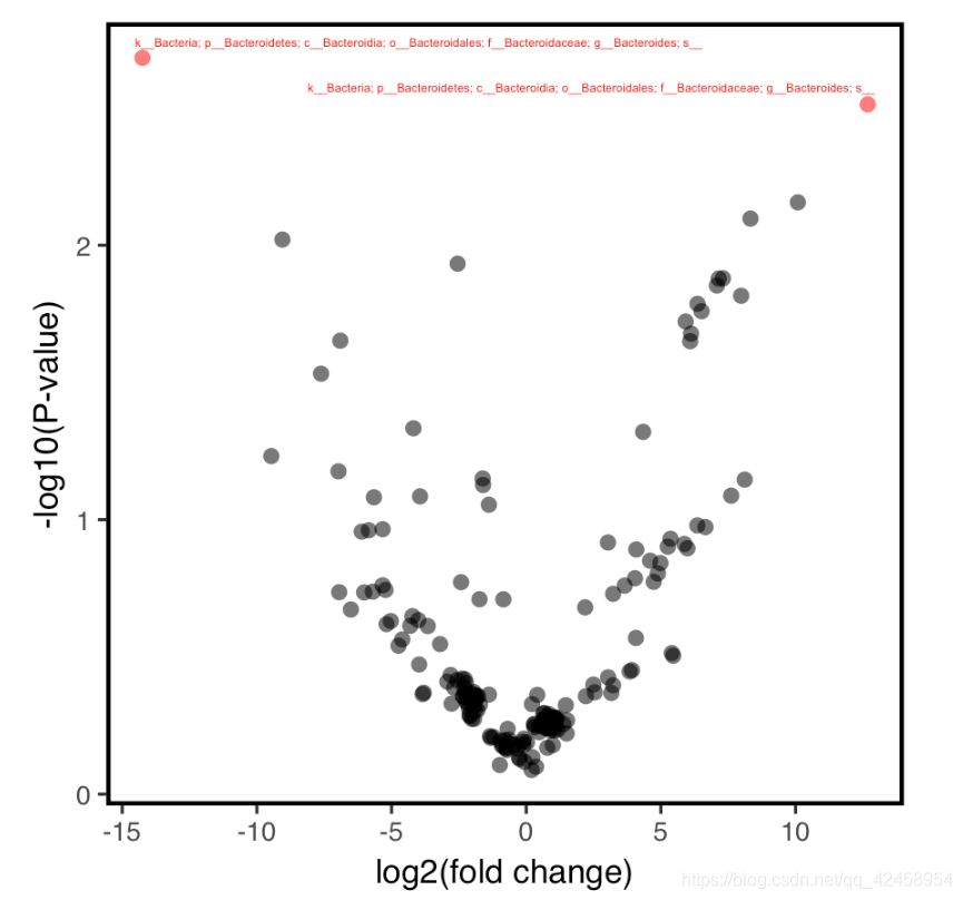
单个feature丰度图
clr<-apply(log2(SVs+0.5), 2, function(x) x-mean(x))
clr %>%
  as.data.frame() %>%
  rownames_to_column("Feature.ID") %>%
  gather(-Feature.ID, key=SampleID, value=CLR) %>%
  filter(Feature.ID=="4b5eeb300368260019c1fbc7a3c718fc") %>%
  left_join(metadata) %>%
  filter(`body-site`=="gut") %>%
  ggplot(aes(x=subject, y=CLR, fill=subject)) +
  stat_summary(geom="bar", color="black") +
  geom_jitter(width=0.2, height=0, shape=21) +
  theme_q2r() +
  theme(legend.position="none")
ggsave("aldexbar.pdf", height=2, width=1.5, device="pdf") 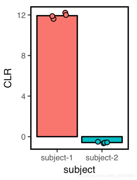
进化树绘制
results<-results %>% mutate(Significant=if_else(we.eBH<0.1,"*", ""))

tree<-drop.tip(tree, tree$tip.label[!tree$tip.label %in% results$Feature.ID]) # remove all the features from the tree we do not have data for
ggtree(tree, layout="circular") %<+% results +
  geom_tippoint(aes(fill=diff.btw), shape=21, color="grey50")  +
  geom_tiplab2(aes(label=Significant), size=10) +
  scale_fill_gradient2(low="darkblue",high="darkred", midpoint = 0, mid="white", name="log2(fold-change") +
  theme(legend.position="right")
ggsave("tree.pdf", height=10, width=10, device="pdf", useDingbats=F) 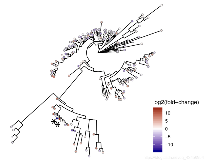


 被折叠的 条评论
为什么被折叠?
被折叠的 条评论
为什么被折叠?
 到【灌水乐园】发言


