气球图R实现(ggballoonplot)

library(ggpubr)
# Define color palette
my_cols <- c("#0D0887FF", "#6A00A8FF", "#B12A90FF",
             "#E16462FF", "#FCA636FF", "#F0F921FF")
# Standard contingency table
#:::::::::::::::::::::::::::::::::::::::::::::::::::::::::
# Read a contingency table: housetasks
# Repartition of 13 housetasks in the couple
data <- read.delim(
  system.file("demo-data/housetasks.txt", package = "ggpubr"),
  row.names = 1
)
data

           Wife Alternating Husband Jointly
Laundry     156          14       2       4
Main_meal   124          20       5       4
Dinner       77          11       7      13
Breakfeast   82          36      15       7
Tidying      53          11       1      57
Dishes       32          24       4      53
Shopping     33          23       9      55
Official     12          46      23      15
Driving      10          51      75       3
Finances     13          13      21      66
Insurance     8           1      53      77
Repairs       0           3     160       2
Holidays      0           1       6     153

# Basic ballon plot
ggballoonplot(data)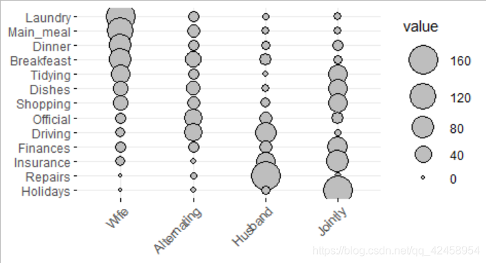

 

# Change color and fill
ggballoonplot(data, color = "#0073C2FF", fill = "#0073C2FF")

 改变颜色

# Change color according to the value of table cells
ggballoonplot(data, fill = "value")+
  scale_fill_gradientn(colors = my_cols)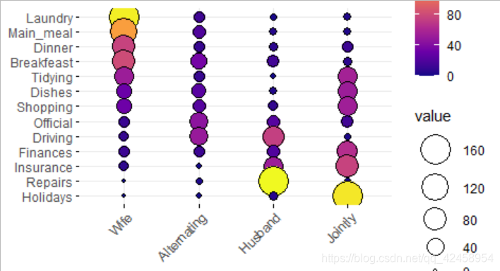

 

改变形状 

# Change the plotting symbol shape
ggballoonplot(data, fill = "value", shape = 23)+
  gradient_fill(c("blue", "white", "red"))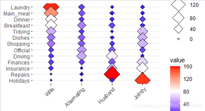

 # Set points size to 8, but change fill color by values
# Sow labels
ggballoonplot(data, fill = "value", color = "lightgray",
              size = 10, show.label = TRUE)+
  gradient_fill(c("blue", "white", "red"))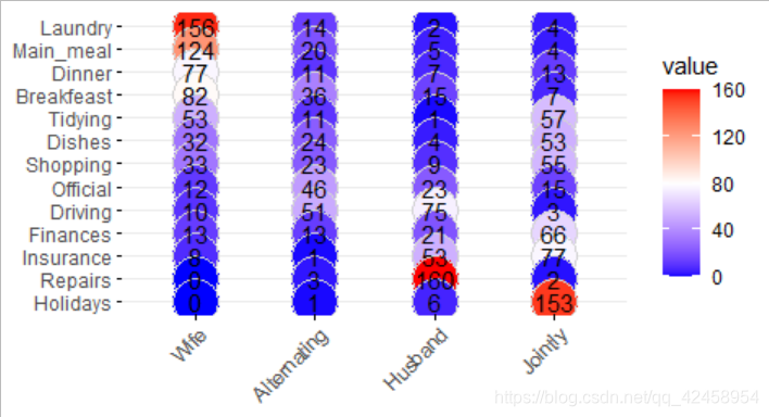

 

# Streched contingency table
#:::::::::::::::::::::::::::::::::::::::::::::::::::::::::
# Create an Example Data Frame Containing Car x Color data
carnames <- c("bmw","renault","mercedes","seat")
carcolors <- c("red","white","silver","green")
datavals <- round(rnorm(16, mean=100, sd=60),1)
car_data <- data.frame(Car = rep(carnames,4),
                       Color = rep(carcolors, c(4,4,4,4) ),
                       Value=datavals )
car_data

        Car  Color Value
1       bmw    red  79.7
2   renault    red  51.2
3  mercedes    red 134.3
4      seat    red  58.5
5       bmw  white 181.9
6   renault  white  12.8
7  mercedes  white 197.5
8      seat  white  82.2
9       bmw silver  49.3
10  renault silver  10.9
11 mercedes silver  91.4
12     seat silver 150.4
13      bmw  green 195.6
14  renault  green 180.4
15 mercedes  green 166.7
16     seat  green 126.9

ggballoonplot(car_data, x = "Car", y = "Color",
              size = "Value", fill = "Value") +
  scale_fill_gradientn(colors = my_cols) +
  guides(size = FALSE)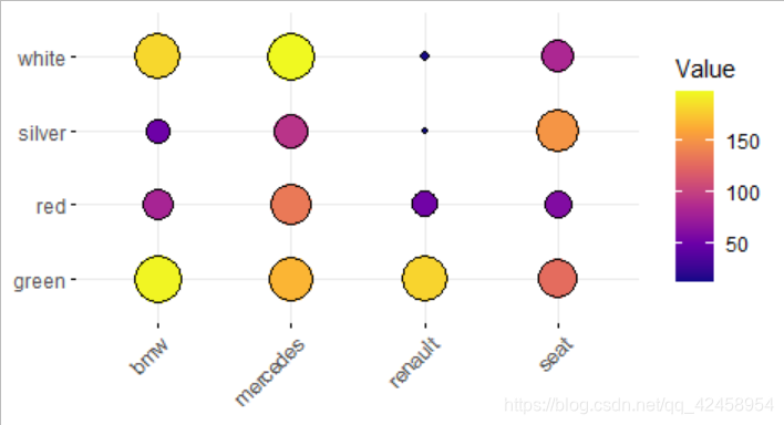

# Grouped frequency table
#:::::::::::::::::::::::::::::::::::::::::::::::::::::::::
data("Titanic")
dframe <- as.data.frame(Titanic)
head(dframe)

  Class    Sex   Age Survived Freq
1   1st   Male Child       No    0
2   2nd   Male Child       No    0
3   3rd   Male Child       No   35
4  Crew   Male Child       No    0
5   1st Female Child       No    0
6   2nd Female Child       No    0

ggballoonplot(
  dframe, x = "Class", y = "Sex",
  size = "Freq", fill = "Freq",
  facet.by = c("Survived", "Age"),
  ggtheme = theme_bw()
)+
  scale_fill_gradientn(colors = my_cols)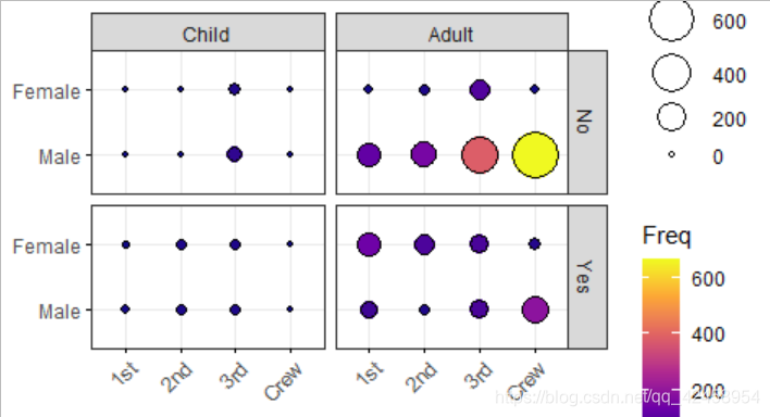

# Hair and Eye Color of Statistics Students32 ggbarplot
data(HairEyeColor)
ggballoonplot( as.data.frame(HairEyeColor),
               x = "Hair", y = "Eye", size = "Freq",
               ggtheme = theme_gray()) %>%
  facet("Sex")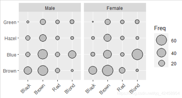

 

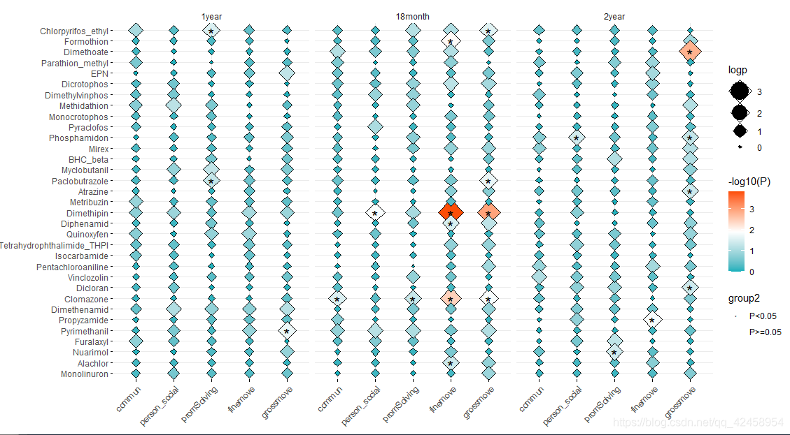
 以我自己数据为例

head(data_plot)

     Outcome             Pesticides  Time Method  time logp  group2
1024  commun Chlorpyrifos_ethyl_log 1year    ASQ 1year 1.03 P>=0.05
1025  commun         Dimethipin_log 1year    ASQ 1year 0.79 P>=0.05
1026  commun         Formothion_log 1year    ASQ 1year 0.16 P>=0.05
1027  commun         Dimethoate_log 1year    ASQ 1year 0.20 P>=0.05
1028  commun         Diphenamid_log 1year    ASQ 1year 0.21 P>=0.05
1029  commun              Mirex_log 1year    ASQ 1year 0.26 P>=0.05

  data_plot$Time<-ordered(data_plot$Time,levels=c("1year","18month","2year"))
  ggballoonplot(data_plot, x = "Time",y = "Pesticides",fill = "logp",
                shape=23,
                #show.label = T,
                size = "logp")+#,
    geom_point(aes(shape=group2,size=1))+
    scale_shape_manual(values=c("*", ""))+
    # facet.by = c("Outcome"))+
    # scale_fill_viridis_c(option = "C")+
    # scale_color_gradient(low="#00AFBB",high = "#FC4E07")+
    gradient_fill(c("#00AFBB", "white", "#FC4E07"))+
    #scale_color_discrete()+
    scale_y_discrete(limits=rev(pes_name),labels=rev(pes_name2))+
    scale_x_discrete(limits=c("1year","18month","2year"))+
    facet_wrap(~ Outcome, ncol=5)+
    labs(fill="-log10(P)")

 Reference:

Ballon plot — ggballoonplot • ggpubr (datanovia.com)