[CAN] [CVPR2019]：Context-Aware Crowd Counting论文+代码解读

行走的人参

已于 2022-07-14 16:46:32 修改

阅读量2.6k

点赞数 1

分类专栏：人群计数文章标签： pycharm 神经网络计算机视觉

于 2022-07-14 16:45:11 首次发布

本文链接：https://blog.csdn.net/qq_42499501/article/details/125784181

版权

人群计数专栏收录该内容

11 篇文章 15 订阅

订阅专栏

1.论文

论文链接：https://arxiv.org/pdf/1811.10452.pdf

代码链接：GitHub - weizheliu/Context-Aware-Crowd-Counting: Official Code for Context-Aware Crowd Counting. CVPR 2019

代码比较简单，我直接看没复现，复现看另外一篇文章。[CAN] Context-Aware Crowd Counting 复现过程记录_wpw5499的博客-CSDN博客

参考：人群计数[CAN]（Context-AwareCrowdCounting）代码解读 - 百度文库

[Crowd_Counting]-CAN-CVPR2019 - 知乎

2.摘要

以往全卷积网络对一张图片的不同地方，都是用了相同尺度的卷积核，感受野都一样，这样无差别对待是有问题的，所以需要让不同人头大小的尺度的信息反应到特征中来，不同的是，通过检测出feature中的细节信息作为attention，去优化特征，最终产生融合了尺度信息的context-aware feature。

3.主要内容

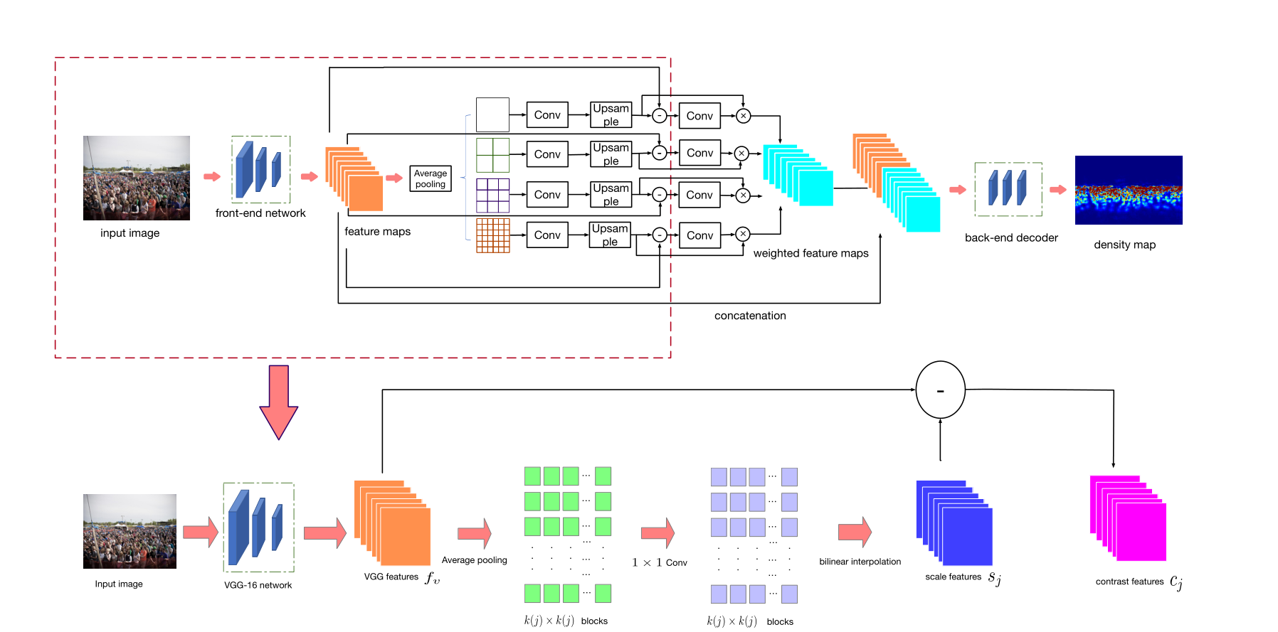
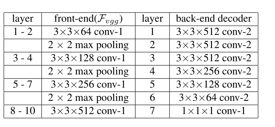
本文的结构其实是一个3段式的结构，front-end, context-aware block,back-end三个部分，front-end跟back-end就是CSRNet的front-end,back-end，跟CSRNet一样，所以本文的方法相当于给CSRNet中间插入了一个context-aware模块。

1.context-aware模块

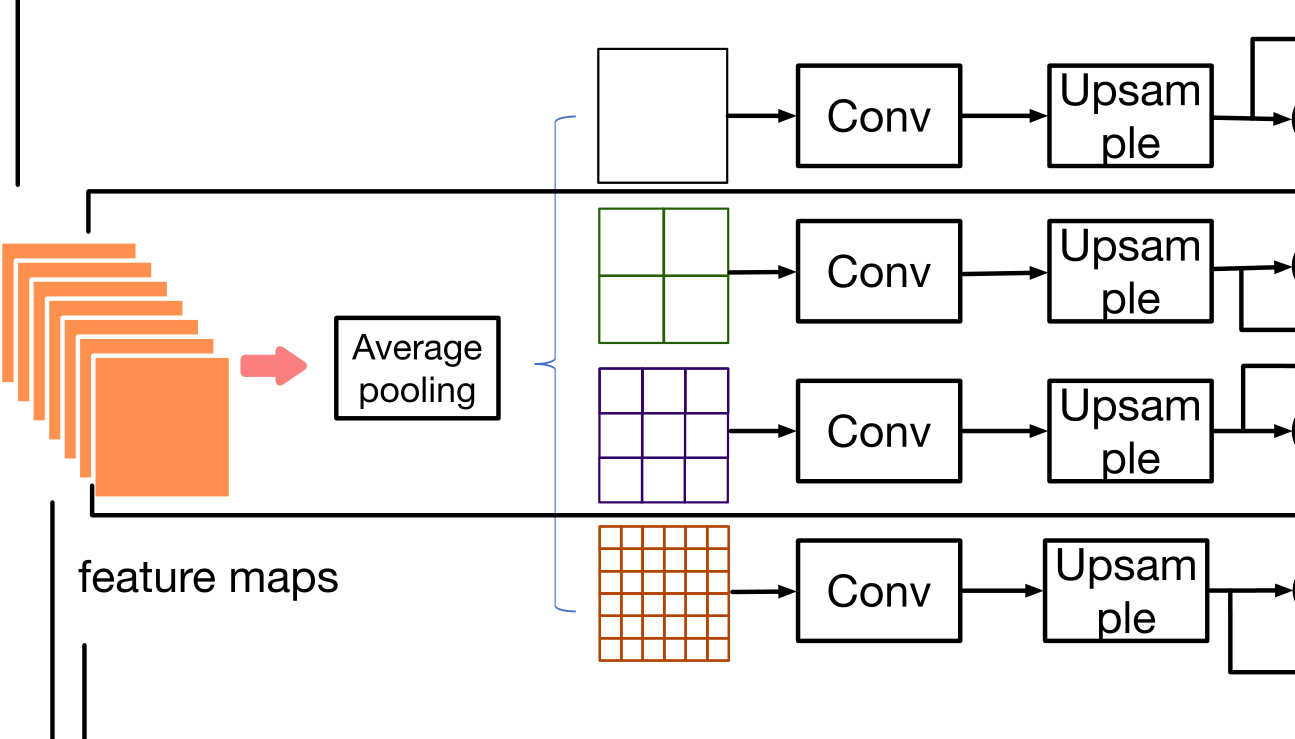
Front-end就是VGG16的前10层，输出512通道的feature，这里称为fv，然后对fv类似于SPP的方法，分成4路，分别用average-pooling分成1x1,2x2,3x3,6x6四种分块方式，然后对每种分块方式经过1x1的卷积，以及bilinear upsampling恢复到fv的尺寸，这种先下采样，再卷积，再上采样恢复出来的feature称为scale-aware。

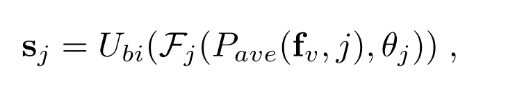
Pave,Fj,Ubi分别表示average pooling，conv，upsampling

对应图中这个部分

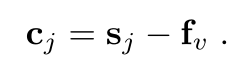
2.Contrast features：

拿backbone的feature fv减去scale-aware feature，就是contrast feature，scale-aware feature是先下采样，再上采样得来的，因此相比于fv丢失了细节，所以constrast则是用fv-sj，就获得了这些丢失的细节，文中说这叫做saliency

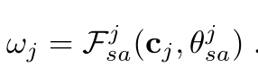
3.Contextual features

将contrast feature cj作为attention，去过滤scale-aware feature sj，具体的做法是cj经过conv和sigmod，获得一个weight map：

然后拿wj跟sj做point-wise乘法，最后4路的feature加起来，最后再跟backbone的feature fv concat起来，形成1024通道的feature，就称为contextual feature：

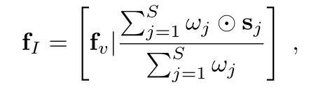
这里[·|·]表示feature的concat操作，最后这个fI就输入back-end

4.融合perspective map的信息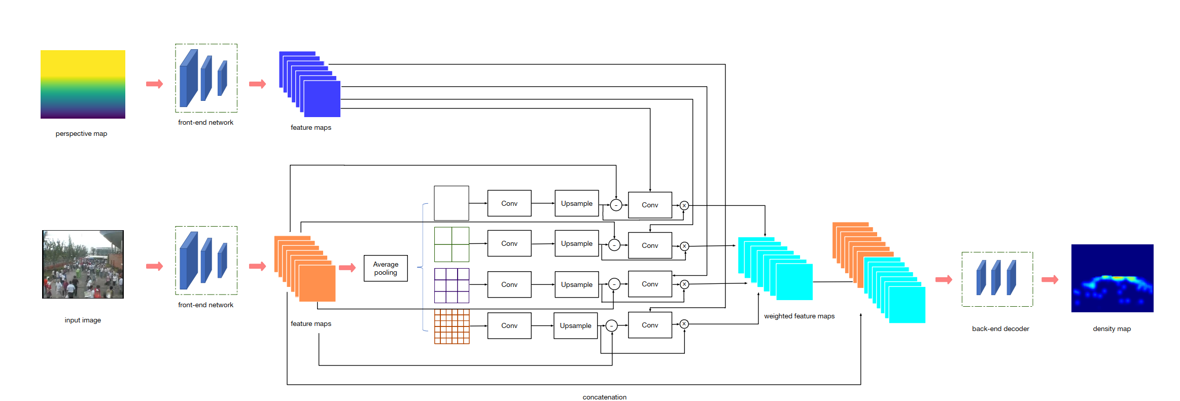

对于存在perspective map的ground truth的dataset，本文尝试把perspective map的信息融合进来，融合的方式是先用VGG16的backbone去提取persepctive的特征fg，然后在求weight map wj时，融入perspective map的feature，做法如下：

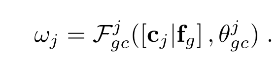
就是把cj跟fg concat起来，再经过conv+sigmod，产生weight map wj，去对scale-aware feature进行相乘，其他方面都不变。

实验

老文章了，实验没什么好看的，直接看消融。

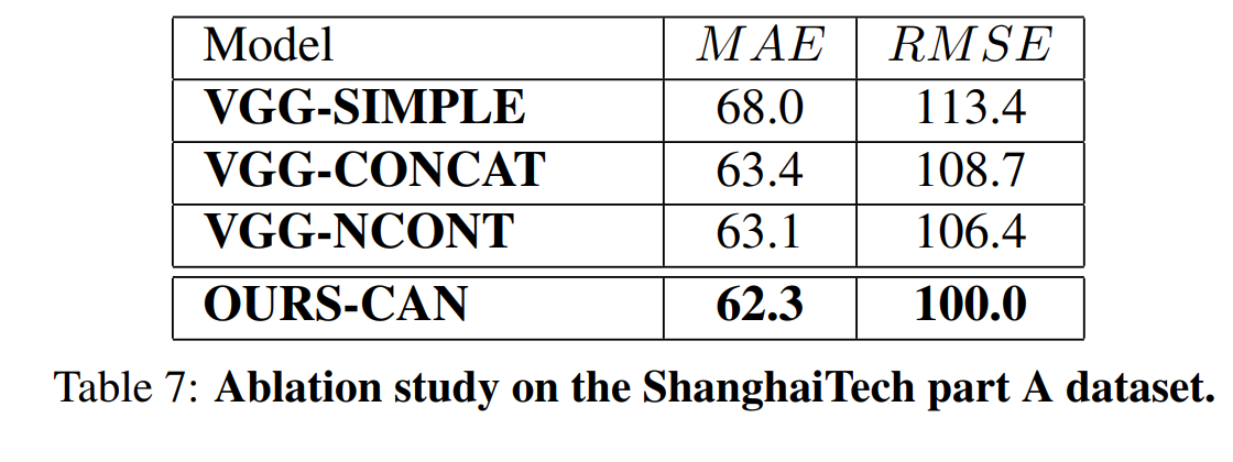
VGG-SIMPLE表示就是直接front-end+back-end，没有中间context-aware模块，其实就是CSRNet，

VGG-CONCAT表示中间模块只把backbone的feature fv跟scale-aware feature sj进行concat，再给back-end，没有计算weight-map对sj进行过滤

VGG-NCONT表示用sj去学习weight map wj，而不是用contrast feature cj去学习weight map，去过滤sj

可见其实巨大的Gain本身来自于加了中间这个模块本身，即可能加了一个SPP模块，contrast feature本身作用不大。

代码

整个网络代码如下：可以看到forward过程中有四个过程，

x = self.frontend(x) # 这就是frontend，即VGG前10层
x = self.context(x)  # 文中提出的中间块
x = self.backend(x)  # VGG的backend
x = self.output_layer(x)  # 1x1的卷积输出。

#本⽂⾃⼰⽹络的模型classCANNet(nn.Module):
def__init__(self,load_weights=False):super(CANNet,self).__init__()self.seen=0
#使⽤前⾯已经建⽴的提取多尺度的上下⽂信息的模型self.context=ContextualModule(512,512)
#⽹络前端，‘M’表⽰这⼀层是⼀个MaxPooling池化层，frontend_feat表⽰的是VGG-16⽹络的前10层self.frontend_feat=[64,64,'M',128,128,'M',256,256,256,'M',512,512,512]
#⽹络后端，back_feat表⽰的是采⽤空洞卷积的后端self.backend_feat=[512,512,512,256,128,64]
#前端和后端都使⽤了make_layers()函数⾃定义实现self.frontend=make_layers(self.frontend_feat)
self.backend=make_layers(self.backend_feat,in_channels=512,batch_norm=True,dilation=True)#最后的output层采⽤了1*1卷积核实现了特征平⾯数量向1的转变。
self.output_layer=nn.Conv2d(64,1,kernel_size=1)#根据前⾯load_weights为False，所以这个if⼀定会执⾏
ifnotload_weights:
#保存VGG-16前10层的⽹络结构mod=models.vgg16(pretrained=True)
#先调⽤self._initialize_weights()⽅法进⾏⼿动初始化self._initialize_weights()
#net.state_dict()是⽹络全部参数的字典，⾥⾯的键是⽹络各层参数的名字，值是封装好参数的Tensor
#dict.items()语句会返回⼀个可遍历的（键，值）元组，通过遍历这个元组的⽅式，即通过逐个的i访问mod.state_dict().items()[i][1].data[:]，即可遍历完所有的参数，完成拷贝。
foriinrange(len(self.frontend.state_dict().items())):list(self.frontend.state_dict().items())[i][1].data[:]=list(mod.state_dict().items())[i][1].data[:]
#对⽹络forward的定义和初始化的⽅法defforward(self,x):
x=self.frontend(x)x=self.context(x)
x=self.backend(x)x=self.output_layer(x)returnx
#net.modules()是⽹络各层的列表，我们使⽤m来遍历列表中的元素，判断m的层类型，然后分别使⽤init下的函数来完成初始化。def_initialize_weights(self):
forminself.modules():
#正态分部：nn.init.normal_(tensor,mean=0,std=1)ifisinstance(m,nn.Conv2d):
nn.init.normal_(m.weight,std=0.01)ifm.biasisnotNone:
nn.init.constant_(m.bias,0)elifisinstance(m,nn.BatchNorm2d):
nn.init.constant_(m.weight,1)nn.init.constant_(m.bias,0)
#⽹络结构⾃定义的函数，是写在类的定义之外的
defmake_layers(cfg,in_channels=3,batch_norm=False,dilation=False):
#通过dilation与否判断空洞率的⼤⼩，若是False则是⽹络前端，空洞率为1，若是True则是⽹络后端，空洞率为2。ifdilation:
d_rate=2else:
d_rate=1layers=[]
#接下来遍历传⼊的frontend_feat和backend_feat，以此来确定⽹络层的类型，若是’M’则是MaxPooling层；
#若是数字，则是卷积层，⼀套卷积层包括了Conv2d层，BatchNorm层和ReLU层，遍历完毕后，即可完成对⽹络前端和后端的创建。
forvincfg:ifv=='M':
layers+=[nn.MaxPool2d(kernel_size=2,stride=2)]else:
conv2d=nn.Conv2d(in_channels,v,kernel_size=3,padding=d_rate,dilation=d_rate)ifbatch_norm:
layers+=[conv2d,nn.BatchNorm2d(v),nn.ReLU(inplace=True)]
else:
#由于batch_norm=False,直接执⾏else语句
layers+=[conv2d,nn.ReLU(inplace=True)]in_channels=v
returnnn.Sequential(*layers)

主要看context阶段：

import torch.nn as nn
import torch
from torch.nn import functional as F
from torchvision import models
#model.py主要实现了对⽹络模型的定义
#提取多尺度的上下⽂信息的模型定义
class ContextualModule(nn.Module):
#我们使⽤S = 4个不同的尺度，对应的块⼤⼩k(j)∈{1,2,3,6}，因为它⽐其他设置表现出更好的性能。
#features是指每个输⼊样本的⼤⼩；out_features是指每个输出样本的⼤⼩；sizes是指尺度⼤⼩
def __init__(self, features, out_features=512, sizes=(1, 2, 3, 6)):
super(ContextualModule, self).__init__()
self.scales = []

self.scales = nn.ModuleList([self._make_scale(features, size) for size in sizes])
#bottleneck 的作⽤还是⽤更合理的⽅法减少了参数的数量，同时在尽可能不删除关键的特征的情况下
#nn.Conv2d(in_channels, out_channels, kernel_size)作为⼆维卷积的实现；features*2是指输⼊张量的通道数;kernel_size是指卷积核的⼤⼩为1*1
self.bottleneck = nn.Conv2d(features * 2, out_features, kernel_size=1)
#nn.ReLU()为激活函数，也是卷积层
self.relu = nn.ReLU()
#每个这样的⽹络输出⼀个特定⽐例的表单权重图
self.weight_net = nn.Conv2d(features, features, kernel_size=1)
#计算预测权值w的函数
def __make_weight(self, feature, scale_feature):
#原⽂中给出的对⽐特征的计算公式：C_j = S_j - f_j，就是计算出对⽐特征
weight_feature = feature - scale_feature
#Sgimoid函数即形似S的函数，也成为S函数。在机器学习中经常⽤作分类
#sigmoid函数来避免除0
#使⽤self.weight_net()来进⼀步学习尺度感知特征的权值
return F.sigmoid(self.weight_net(weight_feature))
#计算尺度
def _make_scale(self, features, size):
#nn.AdaptiveAvgPool2d()⾃适应平均池化函数
prior = nn.AdaptiveAvgPool2d(output_size=(size, size))
#⼆维卷积
conv = nn.Conv2d(features, features, kernel_size=1, bias=False)
#nn.Sequential()⼀个有序的容器，神经⽹络模块将按照传⼊构造器的顺序依次被添加到计算图中执⾏，
return nn.Sequential(prior, conv)
#反馈给后端⽹络
def forward(self, feats):
h, w = feats.size(2), feats.size(3)
#⾃适应处理，学习计算尺度
multi_scales = [F.upsample(input=stage(feats), size=(h, w), mode='bilinear') for stage in self.scales]
#根据⾃适应处理得到得到尺度来计算权值
weights = [self.__make_weight(feats, scale_feature) for scale_feature in multi_scales]
#利⽤权值来计算上下⽂特征（原⽂的公式（5））
overall_features = [(multi_scales[0]*weights[0]+multi_scales[1]*weights[1]+multi_scales[2]*weights[2]+multi_scales[3]*weights[3])/(weights[0]+weights[
1]+weights[2]+weights[3])]+ [feats]
#进⾏卷积处理
bottle = self.bottleneck(torch.cat(overall_features, 1))
return self.relu(bottle)