【阿旭机器学习实战】【31】股票价格预测案例--线性回归

【阿旭机器学习实战】系列文章主要介绍机器学习的各种算法模型及其实战案例，欢迎点赞，关注共同学习交流。

注:本文模型结果不好，仅做学习参考使用，提供思路。了解数据处理思路,训练模型和预测数值的过程。

1. 读取数据

import numpy as np # 数学计算
import pandas as pd # 数据处理
import matplotlib.pyplot as plt
from datetime import datetime as dt

关注公众号：阿旭算法与机器学习，回复：“ML31”即可获取本文数据集、源码与项目文档，欢迎共同学习交流

df = pd.read_csv('./000001.csv') 

print(np.shape(df))
df.head()

(611, 14)

	date	open	high	close	low	volume	price_change	p_change	ma5	ma10	ma20	v_ma5	v_ma10	v_ma20
0	2019-05-30	12.32	12.38	12.22	12.11	646284.62	-0.18	-1.45	12.366	12.390	12.579	747470.29	739308.42	953969.39
1	2019-05-29	12.36	12.59	12.40	12.26	666411.50	-0.09	-0.72	12.380	12.453	12.673	751584.45	738170.10	973189.95
2	2019-05-28	12.31	12.55	12.49	12.26	880703.12	0.12	0.97	12.380	12.505	12.742	719548.29	781927.80	990340.43
3	2019-05-27	12.21	12.42	12.37	11.93	1048426.00	0.02	0.16	12.394	12.505	12.824	689649.77	812117.30	1001879.10
4	2019-05-24	12.35	12.45	12.35	12.31	495526.19	0.06	0.49	12.396	12.498	12.928	637251.61	781466.47	1046943.98

股票数据的特征

• date：日期
• open：开盘价
• high：最高价
• close：收盘价
• low：最低价
• volume：成交量
• price_change：价格变动
• p_change：涨跌幅
• ma5：5日均价
• ma10：10日均价
• ma20:20日均价
• v_ma5:5日均量
• v_ma10:10日均量
• v_ma20:20日均量

# 将每一个数据的键值的类型从字符串转为日期
df['date'] = pd.to_datetime(df['date'])
# 将日期变为索引
df = df.set_index('date')
# 按照时间升序排列
df.sort_values(by=['date'], inplace=True, ascending=True)
df.tail()

	open	high	close	low	volume	price_change	p_change	ma5	ma10	ma20	v_ma5	v_ma10	v_ma20
date
2019-05-24	12.35	12.45	12.35	12.31	495526.19	0.06	0.49	12.396	12.498	12.928	637251.61	781466.47	1046943.98
2019-05-27	12.21	12.42	12.37	11.93	1048426.00	0.02	0.16	12.394	12.505	12.824	689649.77	812117.30	1001879.10
2019-05-28	12.31	12.55	12.49	12.26	880703.12	0.12	0.97	12.380	12.505	12.742	719548.29	781927.80	990340.43
2019-05-29	12.36	12.59	12.40	12.26	666411.50	-0.09	-0.72	12.380	12.453	12.673	751584.45	738170.10	973189.95
2019-05-30	12.32	12.38	12.22	12.11	646284.62	-0.18	-1.45	12.366	12.390	12.579	747470.29	739308.42	953969.39

# 检测是否有缺失数据 NaNs
df.dropna(axis=0 , inplace=True)
df.isna().sum()

open            0
high            0
close           0
low             0
volume          0
price_change    0
p_change        0
ma5             0
ma10            0
ma20            0
v_ma5           0
v_ma10          0
v_ma20          0
dtype: int64

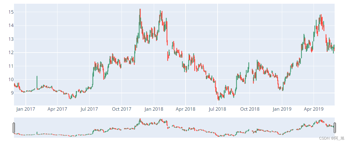
K线图绘制

Min_date = df.index.min()
Max_date = df.index.max()
print ("First date is",Min_date)
print ("Last date is",Max_date)
print (Max_date - Min_date)

First date is 2016-11-29 00:00:00
Last date is 2019-05-30 00:00:00
912 days 00:00:00

from plotly import tools
from plotly.graph_objs import *
from plotly.offline import init_notebook_mode, iplot, iplot_mpl
init_notebook_mode()
import chart_studio.plotly as py
import plotly.graph_objs as go

trace = go.Ohlc(x=df.index, open=df['open'], high=df['high'], low=df['low'], close=df['close'])
data = [trace]
iplot(data, filename='simple_ohlc')

2.构建回归模型

from sklearn.linear_model import LinearRegression
from sklearn import preprocessing

# 创建标签数据：即预测值, 根据当前的数据预测5天以后的收盘价
num = 5 # 预测5天后的情况
df['label'] = df['close'].shift(-num) # 预测值,将5天后的收盘价当作当前样本的标签
                                     
print(df.shape)

(611, 14)

# 丢弃 'label', 'price_change', 'p_change', 不需要它们做预测
Data = df.drop(['label', 'price_change', 'p_change'],axis=1)
Data.tail()

	open	high	close	low	volume	ma5	ma10	ma20	v_ma5	v_ma10	v_ma20
date
2019-05-24	12.35	12.45	12.35	12.31	495526.19	12.396	12.498	12.928	637251.61	781466.47	1046943.98
2019-05-27	12.21	12.42	12.37	11.93	1048426.00	12.394	12.505	12.824	689649.77	812117.30	1001879.10
2019-05-28	12.31	12.55	12.49	12.26	880703.12	12.380	12.505	12.742	719548.29	781927.80	990340.43
2019-05-29	12.36	12.59	12.40	12.26	666411.50	12.380	12.453	12.673	751584.45	738170.10	973189.95
2019-05-30	12.32	12.38	12.22	12.11	646284.62	12.366	12.390	12.579	747470.29	739308.42	953969.39

X = Data.values
# 去掉最后5行，因为没有Y的值
X = X[:-num]
# 将特征进行归一化
X = preprocessing.scale(X)
# 去掉标签为null的最后5行
df.dropna(inplace=True)
Target = df.label
y = Target.values

print(np.shape(X), np.shape(y))

(606, 11) (606,)

# 将数据分为训练数据和测试数据
X_train, y_train = X[0:550, :], y[0:550]
X_test, y_test = X[550:, -51:], y[550:606]
print(X_train.shape)
print(y_train.shape)
print(X_test.shape)
print(y_test.shape)

(550, 11)
(550,)
(56, 11)
(56,)

lr = LinearRegression()
lr.fit(X_train, y_train)
lr.score(X_test, y_test) # 使用绝对系数 R^2 评估模型

0.04930040648385525

# 做预测 ：取最后5行数据，预测5天后的股票价格
X_Predict = X[-num:]
Forecast = lr.predict(X_Predict)
print(Forecast)
print(y[-num:])

[12.5019651  12.45069629 12.56248765 12.3172638  12.27070154]
[12.35 12.37 12.49 12.4  12.22]

# 查看模型的各个特征参数的系数值
for idx, col_name in enumerate(['open', 'high', 'close', 'low', 'volume', 'ma5', 'ma10', 'ma20', 'v_ma5', 'v_ma10', 'v_ma20']):
    print("The coefficient for {} is {}".format(col_name, lr.coef_[idx]))

The coefficient for open is -0.7623399996475224
The coefficient for high is 0.8321435171405448
The coefficient for close is 0.24463705375238926
The coefficient for low is 1.091415550493547
The coefficient for volume is 0.0043807937569128675
The coefficient for ma5 is -0.30717535019465575
The coefficient for ma10 is 0.1935431079947582
The coefficient for ma20 is 0.24902077484698157
The coefficient for v_ma5 is 0.17472336466033722
The coefficient for v_ma10 is 0.08873934447969857
The coefficient for v_ma20 is -0.27910702694420775

3.绘制预测结果

# 预测 2019-05-13 到 2019-05-17 , 一共 5 天的收盘价 
trange = pd.date_range('2019-05-13', periods=num, freq='d')
trange

DatetimeIndex(['2019-05-13', '2019-05-14', '2019-05-15', '2019-05-16',
               '2019-05-17'],
              dtype='datetime64[ns]', freq='D')

# 产生预测值dataframe
Predict_df = pd.DataFrame(Forecast, index=trange)
Predict_df.columns = ['forecast']
Predict_df

	forecast
2019-05-13	12.501965
2019-05-14	12.450696
2019-05-15	12.562488
2019-05-16	12.317264
2019-05-17	12.270702

# 将预测值添加到原始dataframe
df = pd.read_csv('./000001.csv') 
df['date'] = pd.to_datetime(df['date'])
df = df.set_index('date')
# 按照时间升序排列
df.sort_values(by=['date'], inplace=True, ascending=True)
df_concat = pd.concat([df, Predict_df], axis=1)

df_concat = df_concat[df_concat.index.isin(Predict_df.index)]
df_concat.tail(num)

	open	high	close	low	volume	price_change	p_change	ma5	ma10	ma20	v_ma5	v_ma10	v_ma20	forecast
2019-05-13	12.33	12.54	12.30	12.23	741917.75	-0.38	-3.00	12.538	13.143	13.637	1107915.51	1191640.89	1211461.61	12.501965
2019-05-14	12.20	12.75	12.49	12.16	1182598.12	0.19	1.54	12.446	12.979	13.585	1129903.46	1198753.07	1237823.69	12.450696
2019-05-15	12.58	13.11	12.92	12.57	1103988.50	0.43	3.44	12.510	12.892	13.560	1155611.00	1208209.79	1254306.88	12.562488
2019-05-16	12.93	12.99	12.85	12.78	634901.44	-0.07	-0.54	12.648	12.767	13.518	971160.96	1168630.36	1209357.42	12.317264
2019-05-17	12.92	12.93	12.44	12.36	965000.88	-0.41	-3.19	12.600	12.626	13.411	925681.34	1153473.43	1138638.70	12.270702

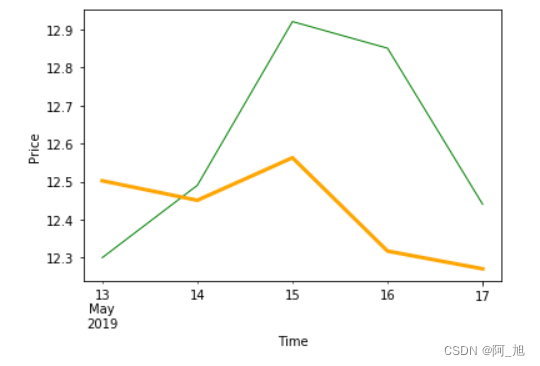
# 画预测值和实际值
df_concat['close'].plot(color='green', linewidth=1)
df_concat['forecast'].plot(color='orange', linewidth=3)
plt.xlabel('Time')
plt.ylabel('Price')
plt.show()

如果文章对你有帮助，感谢点赞+关注！

关注下方GZH：阿旭算法与机器学习，回复：“ML31”即可获取本文数据集、源码与项目文档，欢迎共同学习交流