【三角网】多尺度网格生成（局部加密）

局部加密

• 确保 el1 的最大边长大于 el2 的最大边长
• 确保网格对象按降序排列
• S2区域不使用invert

import matplotlib.gridspec as gridspec
import matplotlib.pyplot as plt
import matplotlib.tri as tri
import numpy as np

import oceanmesh as om

fname = "datasets/bohai/baohai_Polygon.shp"
EPSG = 4326  # EPSG:4326 or WGS84
extent1 = om.Region(extent=(117.00, 124.001, 37.0001, 42.9000), crs=EPSG)
min_edge_length1 = 0.01  # minimum mesh size in domain in projection
bbox2 = np.array(
    [
        [
            119.569110972609,
            38.16619327041994
        ],
        [
            119.569110972609,
            37.846271063325204
        ],
        [
            120.14283882345273,
            37.846271063325204
        ],
        [
            120.14283882345273,
            38.16619327041994
        ],
        [
            119.569110972609,
            38.16619327041994
        ]
    ],
    dtype=float,
)
extent2 = om.Region(extent=bbox2, crs=EPSG)
min_edge_length2 = 0.005  # 加密S2区域的最小网格尺寸

s1 = om.Shoreline(fname, extent1.bbox, min_edge_length1)
sdf1 = om.signed_distance_function(s1, invert=True)
el1 = om.distance_sizing_function(s1, max_edge_length=0.05)

s2 = om.Shoreline(fname, extent2.bbox, min_edge_length2)
sdf2 = om.signed_distance_function(s2)
el2 = om.distance_sizing_function(s2, max_edge_length=0.03)  # 调整最大边长以控制S2区域的加密程度

print("el1 max_edge_length:", el1.dx)
print("el2 max_edge_length:", el2.dx)

# 控制元素大小转换
# from coarse to fine with the kwargs prefixed with `blend`
points, cells = om.generate_multiscale_mesh(
    # [sdf2, sdf1],
    # [el2, el1],
      [sdf1, sdf2],
    [el1, el2],
)
# 删除退化网格面和网格中的其他常见问题
points, cells = om.make_mesh_boundaries_traversable(points, cells)
# 删除单独连接的元素（仅连接到一个其他元素的元素）
points, cells = om.delete_faces_connected_to_one_face(points, cells)
# 去除质量< 15%的不良边界元素
points, cells = om.delete_boundary_faces(points, cells, min_qual=0.15)
# 应用拉普拉斯平滑器来协调网格尺寸分布
points, cells = om.laplacian2(points, cells)

# 绘制它以显示不同级别的分辨率
triang = tri.Triangulation(points[:, 0], points[:, 1], cells)
gs = gridspec.GridSpec(2, 2)
gs.update(wspace=0.5)
plt.figure()

bbox3 = np.array(
    [
        [
            119.39744842569621,
            37.41830070736992
        ],
        [
            119.25660693534473,
            37.34369078100714
        ],
        [
            119.53046538880545,
            37.23163677544504
        ],
        [
            119.6947888819792,
            37.34992179719255
        ],
        [
            119.39744842569621,
            37.41830070736992
        ]
    ],
    dtype=float,
)

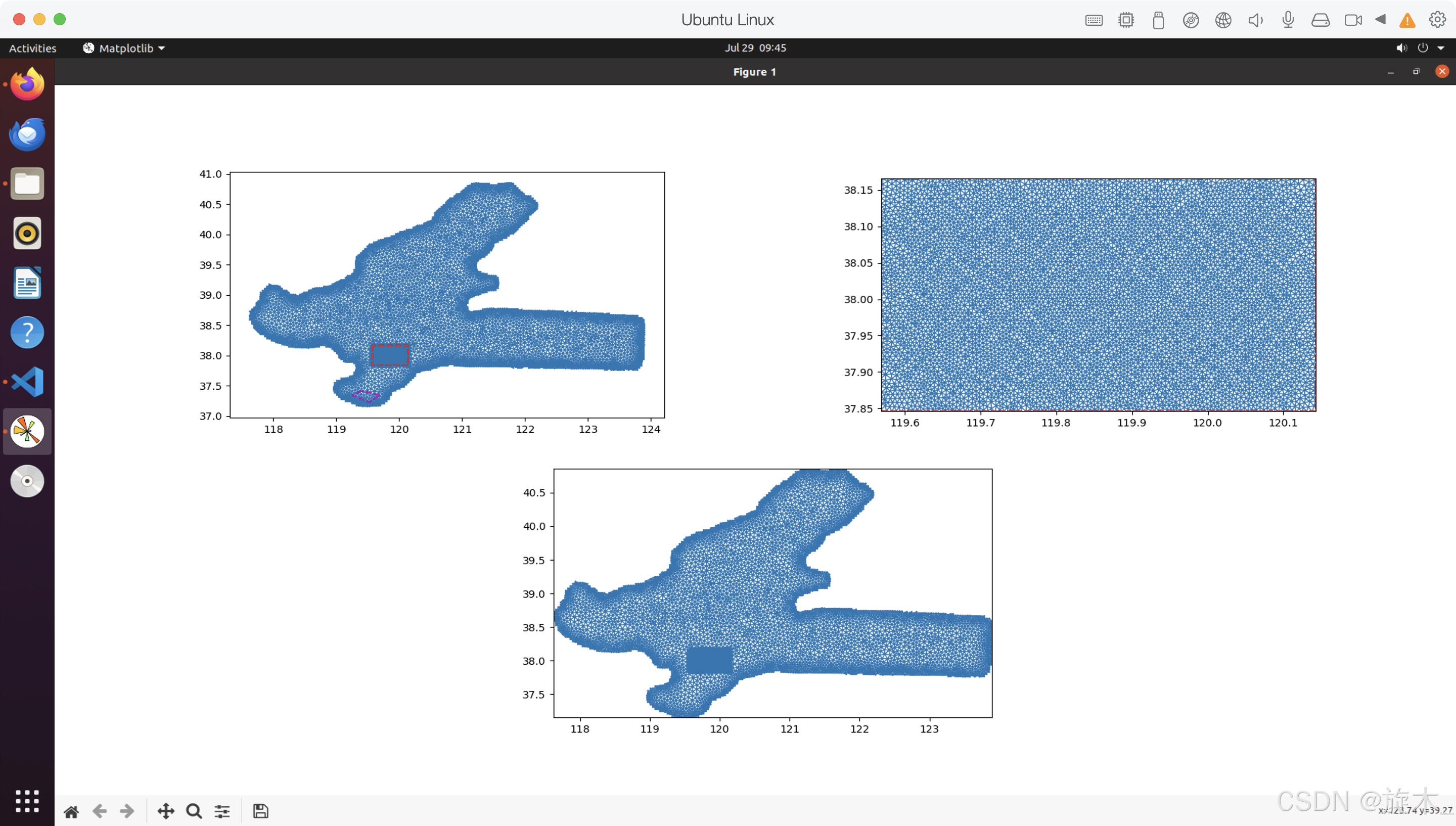
ax = plt.subplot(gs[0, 0])
ax.set_aspect("equal")
ax.triplot(triang, "-", lw=1)
ax.plot(bbox2[:, 0], bbox2[:, 1], "r--")
ax.plot(bbox3[:, 0], bbox3[:, 1], "m--")

ax = plt.subplot(gs[0, 1])
ax.set_aspect("equal")
ax.triplot(triang, "-", lw=1)
ax.plot(bbox2[:, 0], bbox2[:, 1], "r--")
ax.set_xlim(np.amin(bbox2[:, 0]), np.amax(bbox2[:, 0]))
ax.set_ylim(np.amin(bbox2[:, 1]), np.amax(bbox2[:, 1]))
ax.plot(bbox3[:, 0], bbox3[:, 1], "m--")

ax = plt.subplot(gs[1, :])
ax.set_aspect("equal")
ax.triplot(triang, "-", lw=1)
ax.set_xlim(np.amin(points[:, 0]), np.amax(points[:, 0]))
ax.set_ylim(np.amin(points[:, 1]), np.amax(points[:, 1]))
plt.show()

网格生成-区域划分（测试）

import matplotlib.gridspec as gridspec
import matplotlib.pyplot as plt
import matplotlib.tri as tri
import numpy as np

import oceanmesh as om

fname = "datasets/bohai/baohai_Polygon.shp"
EPSG = 4326  # EPSG:4326 or WGS84
extent1 = om.Region(extent=(117.00, 124.001, 37.0001, 42.9000), crs=EPSG)
min_edge_length1 = 0.01  # minimum mesh size in domain in projection
bbox2 = np.array(
    [
      [
              119.569110972609,
              38.16619327041994
            ],
            [
              119.569110972609,
              37.846271063325204
            ],
            [
              120.14283882345273,
              37.846271063325204
            ],
            [
              120.14283882345273,
              38.16619327041994
            ],
            [
              119.569110972609,
              38.16619327041994
            ]
    ],
    dtype=float,
)
extent2 = om.Region(extent=bbox2, crs=EPSG)
min_edge_length2 = 0.02  # minimum mesh size in domain in projection
s1 = om.Shoreline(fname, extent1.bbox, min_edge_length1)
sdf1 = om.signed_distance_function(s1,invert=True)
el1 = om.distance_sizing_function(s1, max_edge_length=0.05)
s2 = om.Shoreline(fname, extent2.bbox, min_edge_length2)
sdf2 = om.signed_distance_function(s2,invert=True)
el2 = om.distance_sizing_function(s2, max_edge_length=0.04)
print("el1 max_edge_length:", el1.dx)
print("el2 max_edge_length:", el2.dx)
# 控制元素大小转换
# from coarse to fine with the kwargs prefixed with `blend`
points, cells = om.generate_multiscale_mesh(
    # [sdf1, sdf2],
    # [el1, el2],
     [sdf2, sdf1],
    [el2, el1],
)
# 删除退化网格面和网格中的其他常见问题
points, cells = om.make_mesh_boundaries_traversable(points, cells)
# 删除单独连接的元素（仅连接到一个其他元素的元素）
points, cells = om.delete_faces_connected_to_one_face(points, cells)
# 去除质量< 15%的不良边界元素
points, cells = om.delete_boundary_faces(points, cells, min_qual=0.15)
# 应用拉普拉斯平滑器来协调网格尺寸分布
points, cells = om.laplacian2(points, cells)

# 绘制它以显示不同级别的分辨率
triang = tri.Triangulation(points[:, 0], points[:, 1], cells)
gs = gridspec.GridSpec(2, 2)
gs.update(wspace=0.5)
plt.figure()

bbox3 = np.array(
    [
       [
              119.39744842569621,
              37.41830070736992
            ],
            [
              119.25660693534473,
              37.34369078100714
            ],
            [
              119.53046538880545,
              37.23163677544504
            ],
            [
              119.6947888819792,
              37.34992179719255
            ],
            [
              119.39744842569621,
              37.41830070736992
            ]
    ],
    dtype=float,
)

ax = plt.subplot(gs[0, 0])  #
ax.set_aspect("equal")
ax.triplot(triang, "-", lw=1)
ax.plot(bbox2[:, 0], bbox2[:, 1], "r--")
ax.plot(bbox3[:, 0], bbox3[:, 1], "m--")

ax = plt.subplot(gs[0, 1])
ax.set_aspect("equal")
ax.triplot(triang, "-", lw=1)
ax.plot(bbox2[:, 0], bbox2[:, 1], "r--")
ax.set_xlim(np.amin(bbox2[:, 0]), np.amax(bbox2[:, 0]))
ax.set_ylim(np.amin(bbox2[:, 1]), np.amax(bbox2[:, 1]))
ax.plot(bbox3[:, 0], bbox3[:, 1], "m--")

ax = plt.subplot(gs[1, :])
ax.set_aspect("equal")
ax.triplot(triang, "-", lw=1)
ax.set_xlim(-73.78, -73.75)
ax.set_ylim(40.60, 40.64)
plt.show()