Cadence的杂碎技巧-学到就更新

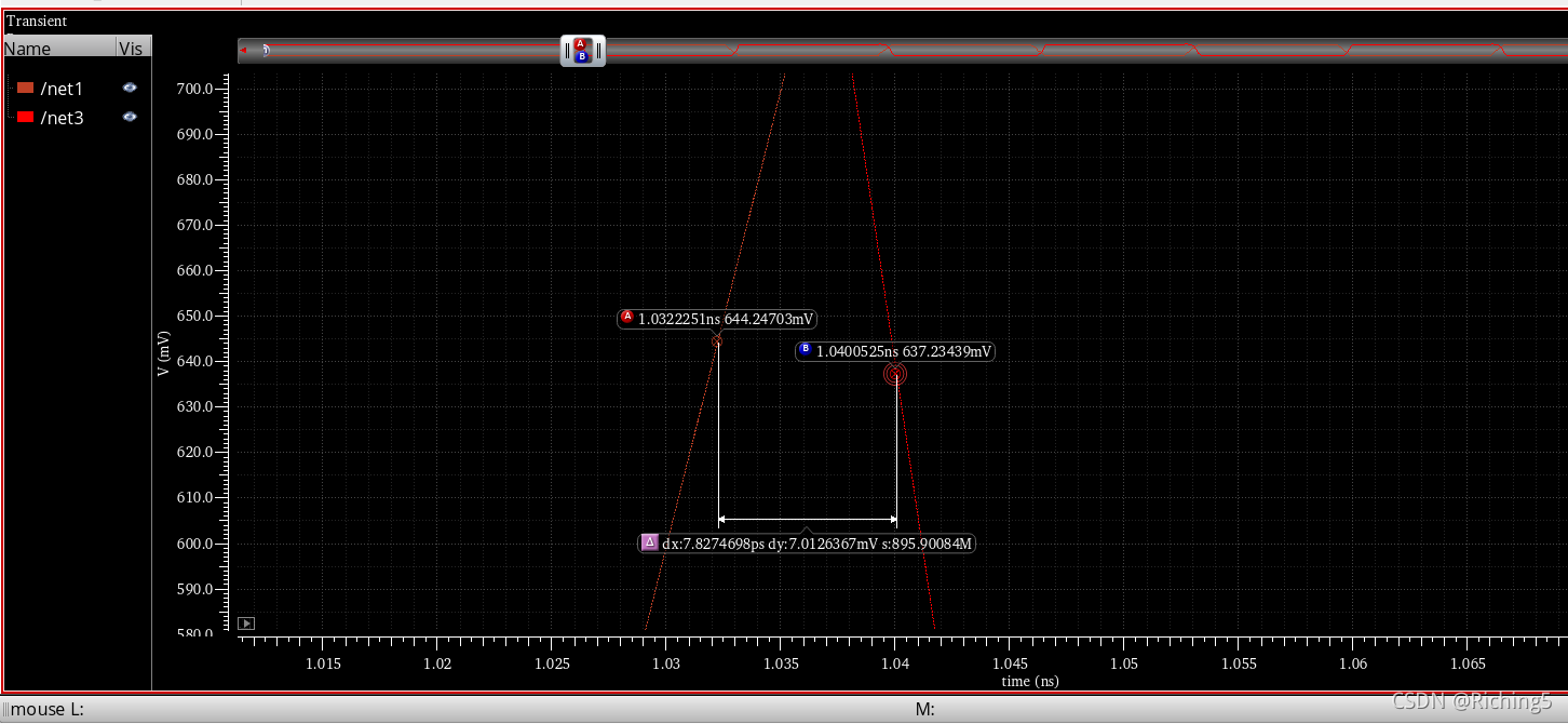
游标放置

将鼠标放在要测曲线附近，按A或B即可添加两个游标

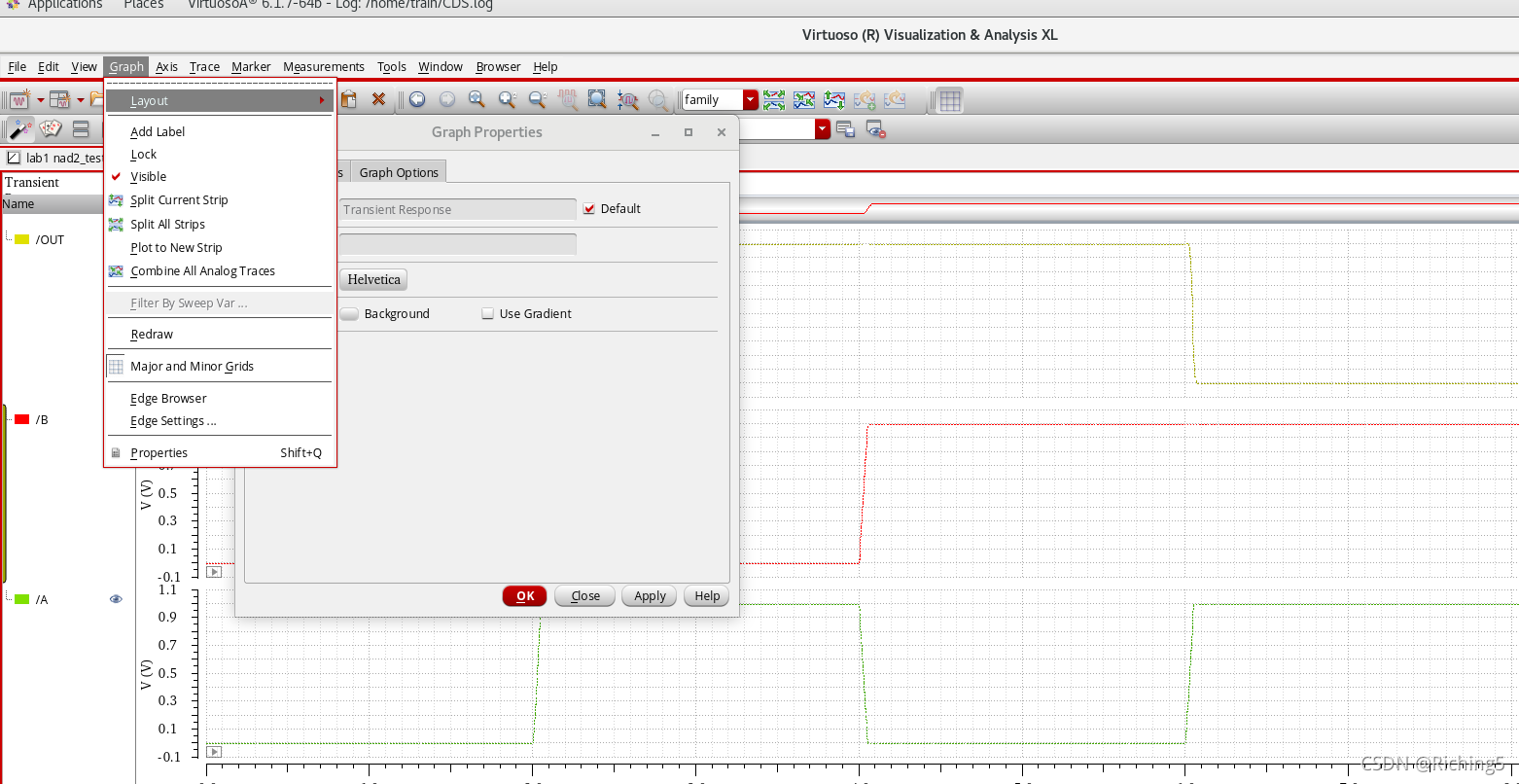
调仿真图背景色

多选元器件

按住shift，再鼠标点击

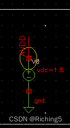
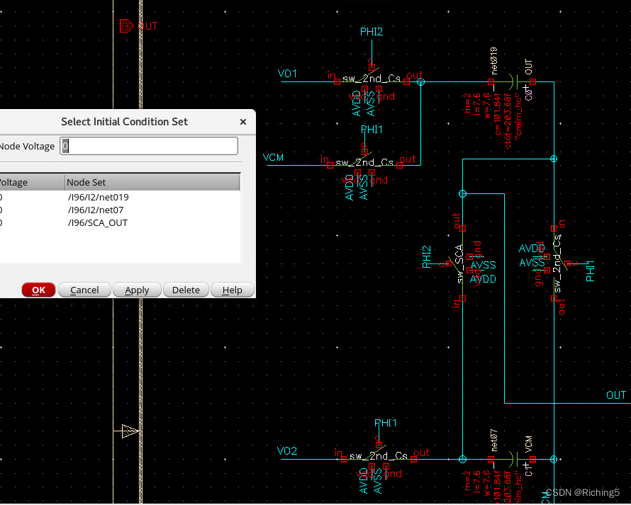
仿真时设置结点电压的初始值

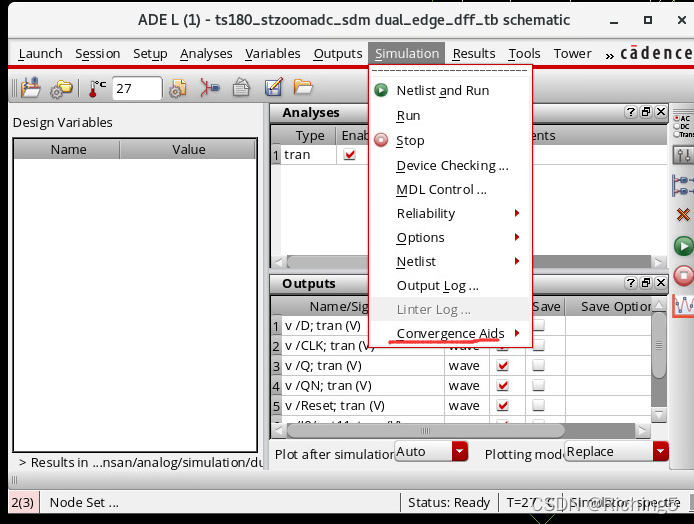
选initial condition，设置一个初始电压
注意：尽管你设计某一结点最开始的电压，但有可能因为其他电路对它的影响而很快变成其他电压值

原理图只读不能编辑

打开原理图–file–make editable

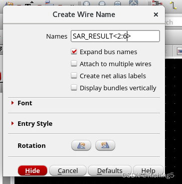
一次创建多个label

空格隔开

方便设置总线label

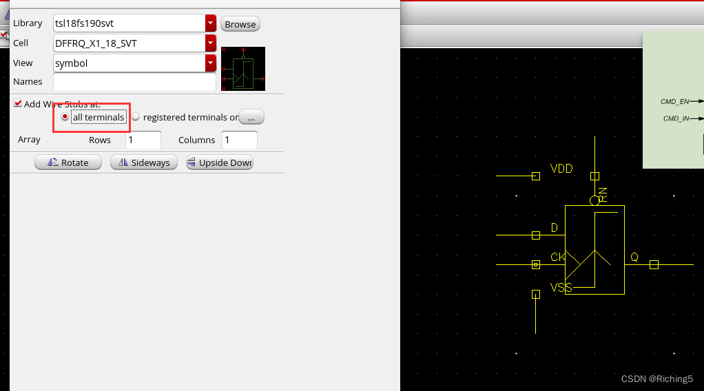
调用元件时生成连线出来

如果选择右边选项，则只会生成设置了端口label名字的线出来

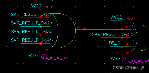
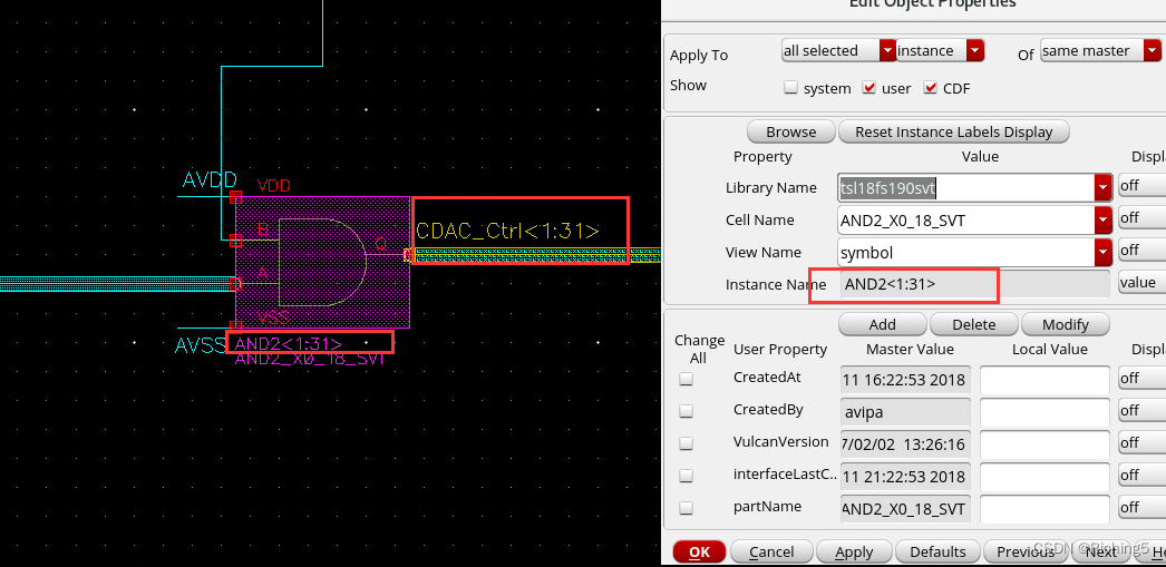
多位宽线路经过同一模块时

可以根据位宽命名器件

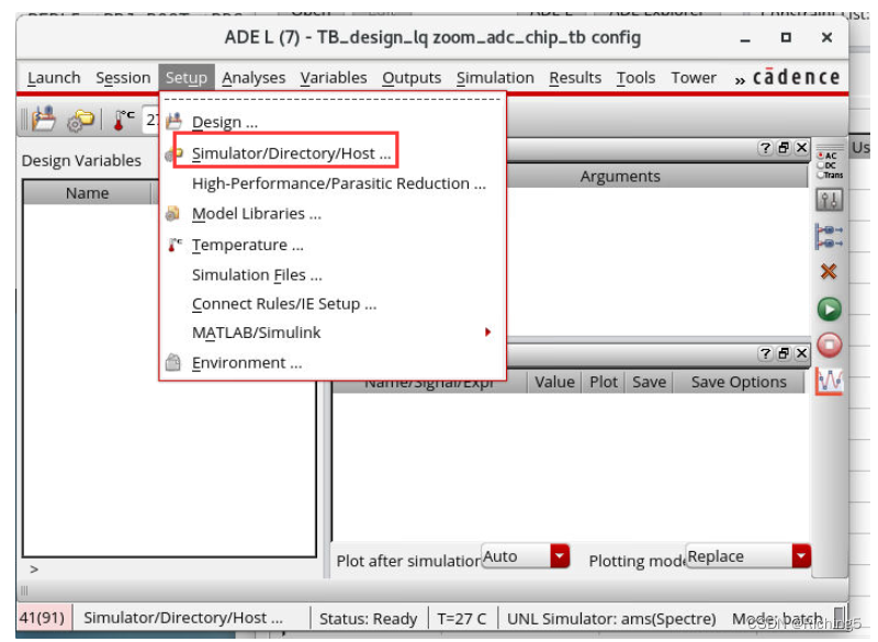
从仿真器打开原理图

电流正负

流入节点为正，流出为负

合并多个端口的pin

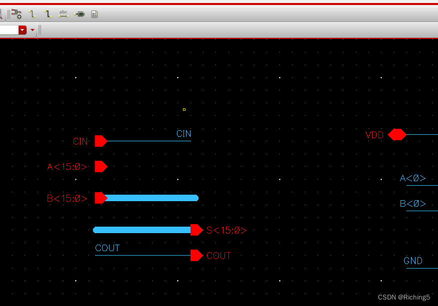
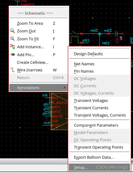
设置annotations

原理图界面右键进入设置

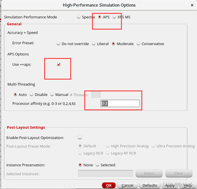
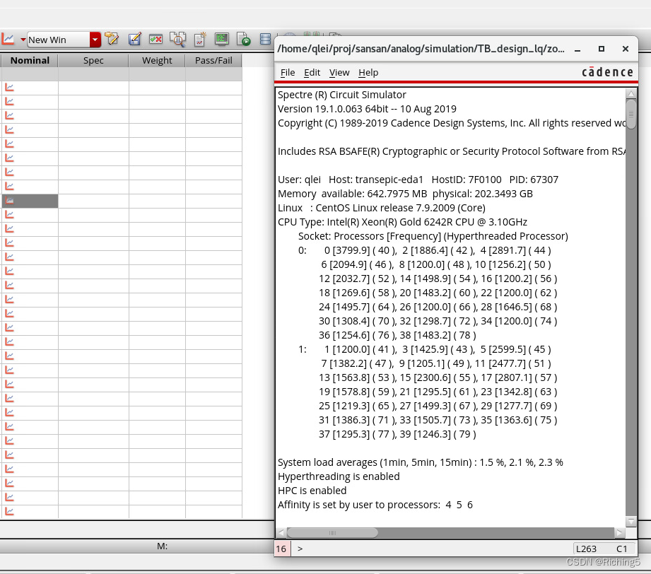
APS 高性能仿真

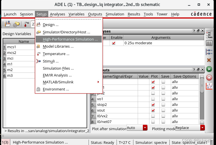
processor affinity应该设置为0-X才是使用X+1个核，如果是当个数字，代表是选第几个核

出现电流震荡的情况

trans时电流与设想的不一样

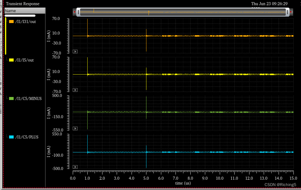
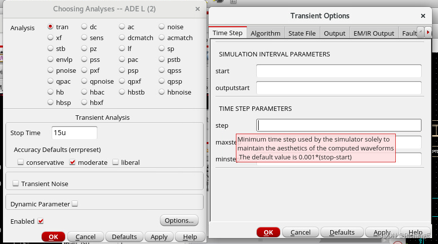
方法一：将仿真步长设置的更小

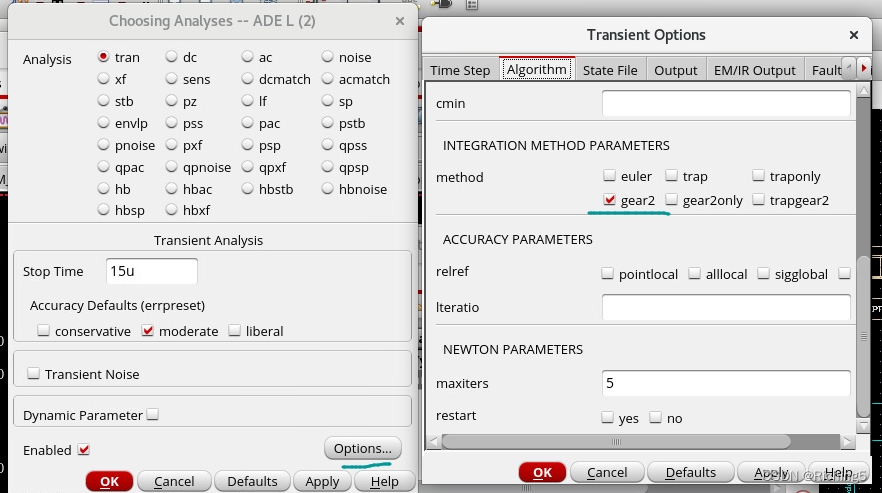
方法2：设置仿真算法
来自外网的回答
Gear method is better than others to get higher accuracy, also in Spectre.
We already know the above in Hspice but it was not clear, at least to me, in Spectre, because it just says ‘default’, but what is the default?, what is his ‘conservative’?
Now I understand that when we scpecify ‘conservative’, then his ‘default’ will be set to ‘gear2only’. Here, also in Spectre, gear is better than others, even though the help file says “trapezoidal is used when we need high accuracy” and “gear can make system more stable than they really are.”

If you used trap or traponly, try and select gear2, gear2only or even euler.
For the differences, study e.g. Kenneth S. Kundert’s book “The Designers Guide to SPICE & SPECTRE”, especially the 4.2.2 chapter on “Characteristics of the Integration Methods” (about 25 pages).
Here just a few clippings: “trapezoidal rule exhibits strong point-to-point ringing.” (p.135); “backward Euler exhibits heavy damping” (p.147); “trapezoidal ringing” (p.150); “To avoid trapezoidal ringing, use Gear2” (p.155).
If you set Spectre’s errpreset property to conservative, the gear2only method is used by default. I’d suggest to use this one first.

更多仿真精度算法介绍
We can refer the help file of Spectre from UNIX command line using :
% spectre -help tran
(thanks José for this tip)
In it, we can find the accuracy comments as follows:

The method' parameter specifies the integration method. The possible settings and their meanings are: method=euler’: Backward-Euler is used exclusively.
method=traponly': Trapezoidal rule is used almost exclusively. method=trap’: Backward-Euler and the trapezoidal rule are used.
method=gear2only': Gear's second-order backward-difference method is used almost exclusively. method=gear2’: Backward-Euler and second-order Gear are used.
`method=trapgear2’: Allows all three integration methods to be used.
The trapezoidal rule is usually the most efficient when you want high accuracy.
This method can exhibit point-to-point ringing, but you can control this by
tightening the error tolerances. For this reason, though, if you choose very
loose tolerances to get a quick answer, either backward-Euler or second-order
Gear will probably give better results than the trapezoidal rule. Second-order
Gear and backward-Euler can make systems appear more stable than they really
are. This effect is less pronounced with second-order Gear or when you request
high accuracy.

Several parameters determine the accuracy of the transient analysis. reltol' and abstol’ control the accuracy of the discretized equation solution. These
parameters determine how well charge is conserved and how accurately steady-
state or equilibrium points are computed. You can set the integration error,
or the errors in the computation of the circuit dynamics (such as time
constants), relative to reltol' and abstol’ by setting the `lteratio’
parameter.

The parameter relref' determines how the relative error is treated. The relref’ options are:
relref=pointlocal': Compares the relative errors in quantities at each node to that node alone. relref=alllocal’: Compares the relative errors at each node to the largest
values found for that node alone for all past time.
relref=sigglobal': Compares relative errors in each of the circuit signals to the maximum for all signals at any previous point in time. relref=allglobal’: Same as relref=sigglobal' except that it also compares the residues (KCL error) for each node to the maximum of that node's past history. The errpreset’ parameter lets you adjust the simulator parameters to fit your
needs quickly. You can set errpreset' to conservative’ if the circuit is
very sensitive, or you can set it to liberal' for a fast. but possibly inaccurate, simulation. The setting errpreset=moderate’ suits most needs.

The effect of errpreset' on other parameters is shown in the following table. In this table, T’= stop' - start’.
errpreset reltol relref method maxstep lteratio

liberal * 10 allglobal gear2 Interval/10 3.5
moderate sigglobal traponly Interval/50 3.5
conservative * 0.1 alllocal gear2only Interval/100 10.0

The value of reltol' is increased or decreased from its value in the options statement, but it is not allowed to be larger than 0.01. Spectre sets the value of maxstep’ so that it is no larger than the value given in the table. Except
for reltol' and maxstep’, `errpreset’ does not change the value of any
parameters you have explicitly set. The actual values used for the transient
analysis are given in the log file.

If the circuit you are simulating can have infinitely fast transitions (for
example, a circuit that contains nodes with no capacitance), Spectre might have
convergence problems. To avoid this, you must prevent the circuit from
responding instantaneously. You can accomplish this by setting `cmin’, the
minimum capacitance to ground at each node, to a physically reasonable nonzero
value. This often significantly improves Spectre convergence.

Spectre provides two methods for reducing the number of output data points
saved: strobing', based on the simulation time, and skipping’ time points,
which saves only every N’th point.

The parameters strobeperiod' and strobedelay’ control the strobing
method.strobeperiod' sets the interval between points that you want to save, and strobedelay’ sets the offset within the period relative to `skipstart’.
The simulator forces a time step on each point to be saved, so the data is
computed, not interpolated.

The skipping method is controlled by `skipcount’. If this is set to N, then
only every N’th point is saved.

The parameters skipstart' and skipstop’ apply to both data reduction methods.
Before skipstart' and after skipstop’, Spectre saves all computed data.

If you do not want any data saved before a given time, use outputstart'. If you do not want any data saved after a given time, change the stop’ time.

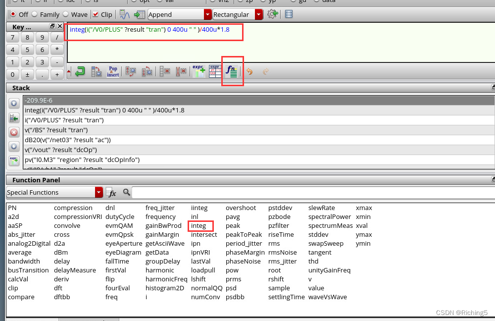
计算电源平均功耗

plot电源负端电流（这里选错了）送到计算器

对电流在仿真时间里积分然后除以仿真时间乘以vdd

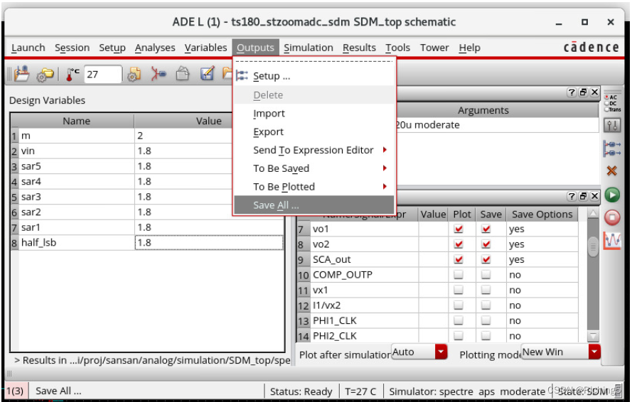
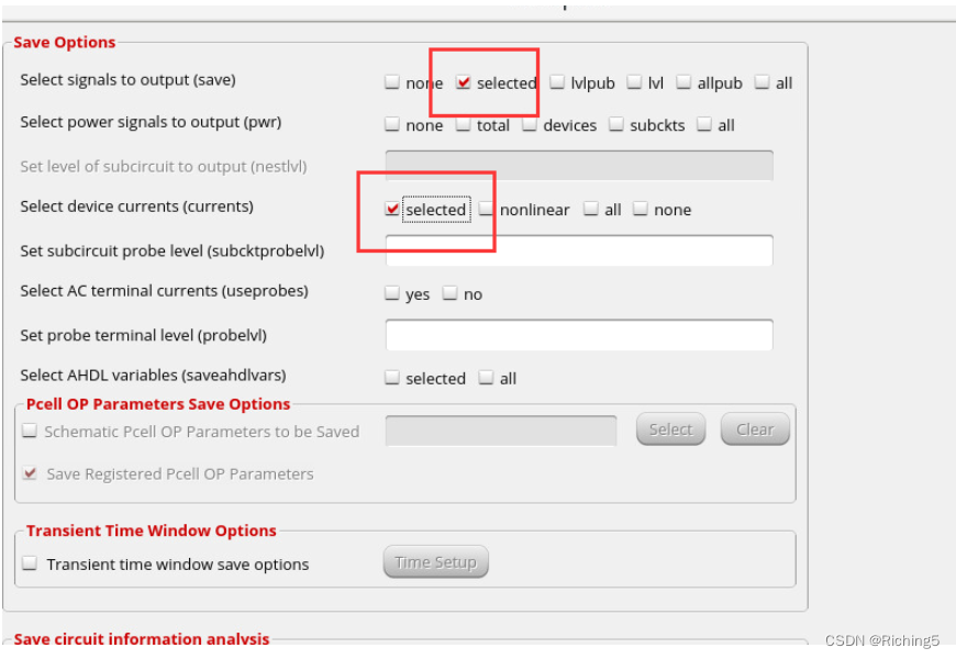
提高仿真速度

仿真提速：把save里改为selected

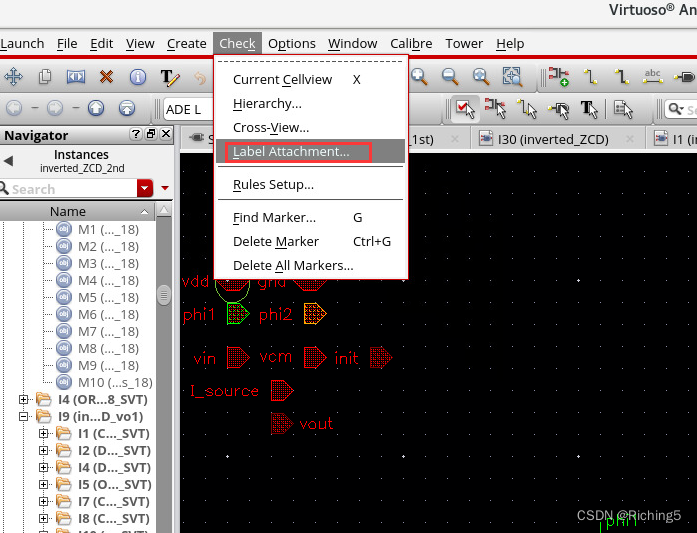
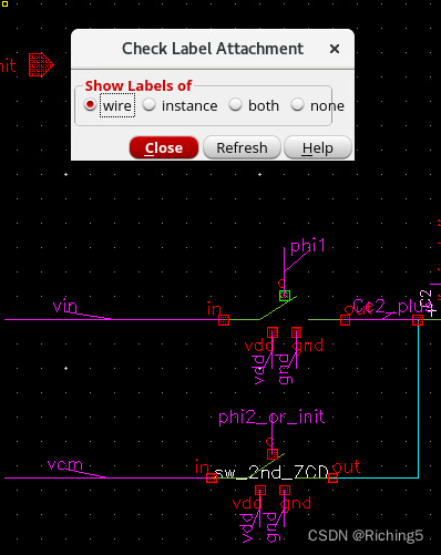
检查label的连接情况

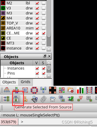
生成指定原理图中模块的版图

点击后点击原理图中模块

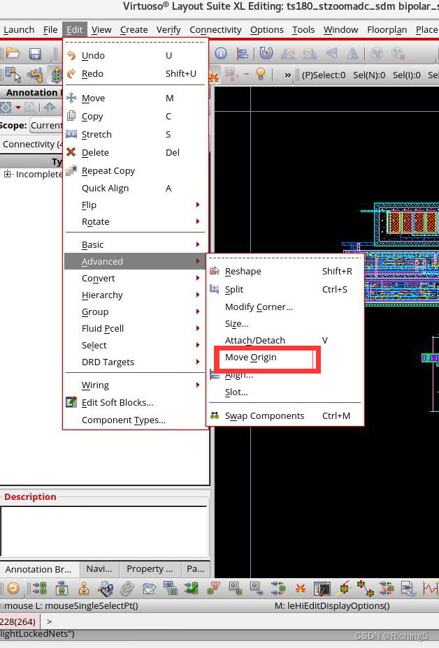
放置版图的坐标轴

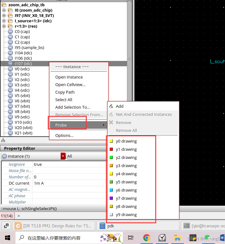
给电路放置探针

用于版图时点亮指定net

仿真无法收敛

如果发生的点在电容两侧，可能是在初始时电容两侧有悬空的端口，所以给无法收敛的点加个初始电压
输入节点电压，然后直接点图中线

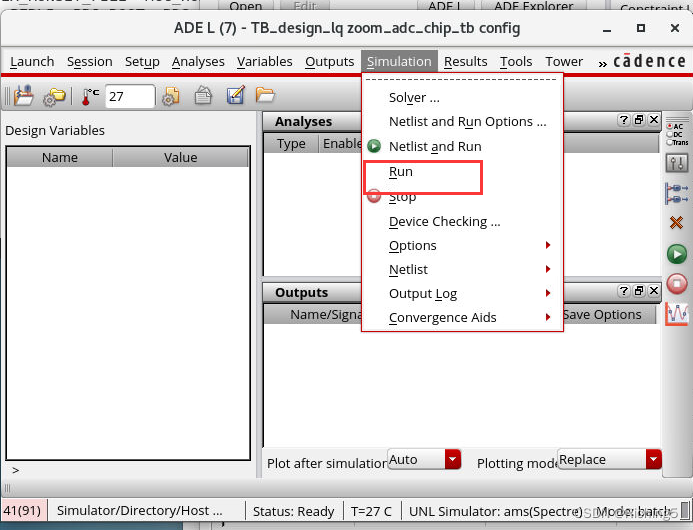
切换仿真器类型

跑别的电路的网表

copy别的电路网表到当前电路simulation里放netlist的位置作替换，然后只run仿真器

一个电路原理图同时跑两个仿真

使用ADEXL然后添加多个tb

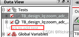
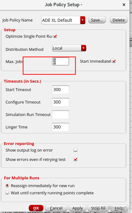
将job设置为2

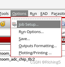
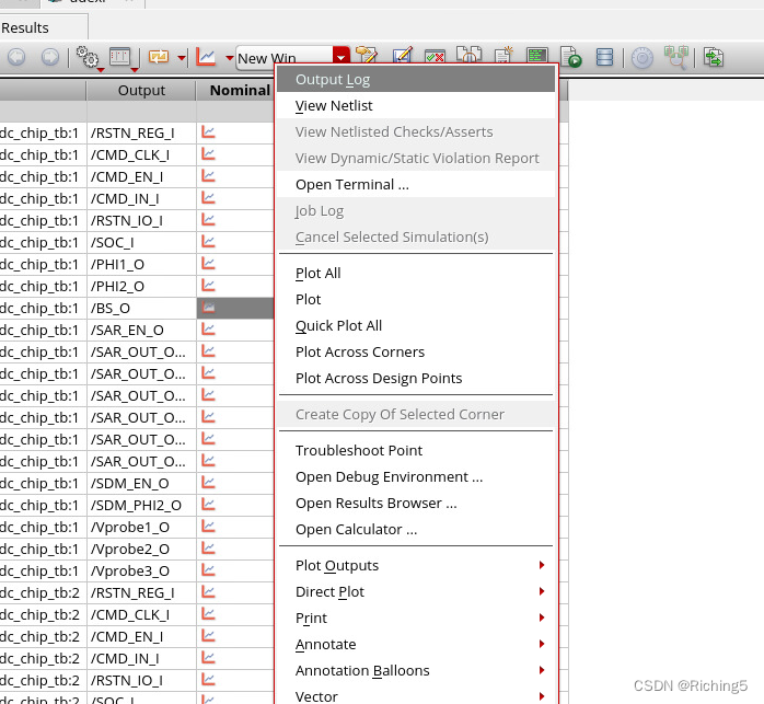
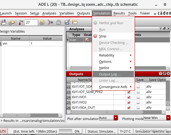
在ADEXL里查看仿真日志

选择Detail

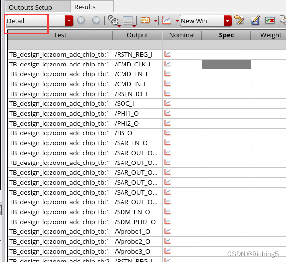
右键一个仿真，点Output Log

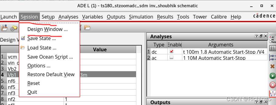
重新打开ADEXL里已经关闭的仿真结果

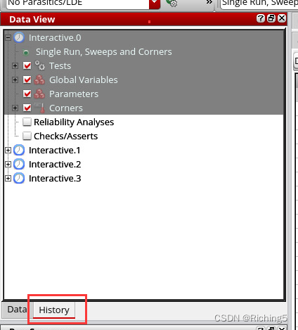
在ADEL打开仿真日志

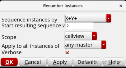
排序器件

Edit -> Renumber Instances
X+Y+：先从左到右再从下往上编号