在没有深度学习的情况下找到道路

点击上方“小白学视觉”，选择加"星标"或“置顶”

重磅干货，第一时间送达

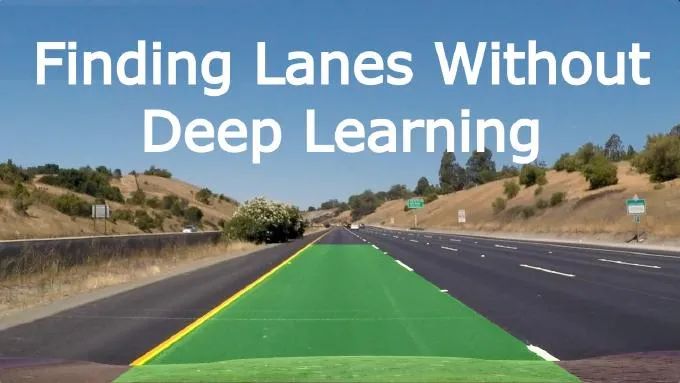
今天我们将一起参与一个项目，使用python在图像和视频中找到车道。对于该项目，我们将采用手动方法。尽管我们确实可以使用深度学习等技术获得更好的结果，但学习概念、工作原理和基础知识也很重要，这样我们在构建高级模型时就可以应用我们已经学到的知识。在使用深度学习时，可能还需要我们介绍的一些步骤。

我们将采取的步骤如下：

• 计算相机校准并解决失真。

• 应用透视变换来校正二值图像（“鸟瞰图”）。

• 使用颜色变换、渐变等来创建阈值二值图像。

• 检测车道像素并拟合以找到车道边界。

• 确定车道的曲率和车辆相对于中心的位置。

• 将检测到的车道边界变形回原始图像。

• 输出车道边界的视觉显示以及车道曲率和车辆位置的数值估计。

所有代码和解释都可以在我们的Github 中找到 。

计算相机校准

今天的廉价针孔相机给图像带来了很多失真，两种主要的畸变是径向畸变和切向畸变。

由于径向畸变，直线会显得弯曲，当我们远离图像的中心时，它的影响更大。例如，如下图所示，棋盘的两个边缘用红线标记，但是我们可以看到边框不是一条直线，并且与红线不匹配。所有预期的直线都凸出来了。

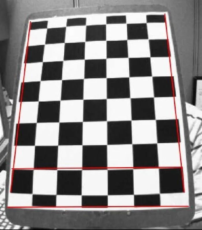相机失真示例

为了解决这个问题，我们将使用OpenCV python 库，并使用目标相机拍摄的示例图像来制作棋盘。为什么是棋盘？在棋盘图像中，我们可以很容易地测量失真，因为我们知道物体的外观，我们可以计算从源点到目标点的距离，并使用它们来计算失真系数，然后使用这些系数来修复图像。

下图显示了来自输出图像和未失真结果图像的示例：

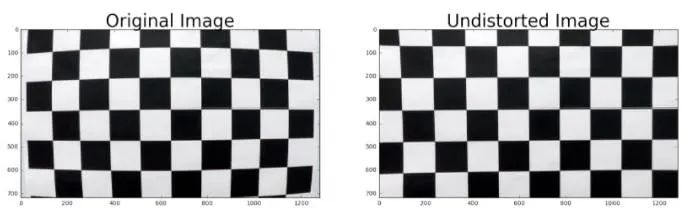修复相机失真

（所有这些效果都发生在lib/camera.py文件中），但它是如何工作的？该过程包括 3 个步骤：

对图像进行采样：

在这一步中，我们识别定义棋盘格的角点，以防我们找不到棋盘，或者棋盘不完整，我们将丢弃样本图像。

# first we convert the  image to grayscale
gray = cv2.cvtColor(img, cv2.COLOR_BGR2GRAY)


# Find the chessboard corners
ret, corners = cv2.findChessboardCorners(gray, (9, 6), None)

校准：

在这一步中，我们从校准模式的多个视图中找到相机的内在和外在参数，然后我们可以使用它们来生成结果图像。

img_size = (self._valid_images[0].shape[1], self._valid_images[0].shape[0])
ret, self._mtx, self._dist, t, t2 = cv2.calibrateCamera(self._obj_points, self._img_points, img_size, None, None)

不失真：

在这最后一步中，我们实际上通过根据校准步骤中检测到的参数补偿镜头失真来生成最终图像。

cv2.undistort(img, self._mtx, self._dist, None, self._mtx)

应用透视变换来校正二值图像（“鸟瞰图”）。

该过程的下一步是更改图像的视角，从安装在汽车前部的常规摄像头视图变为俯视图，也称为“鸟瞰图”。这是它的样子：

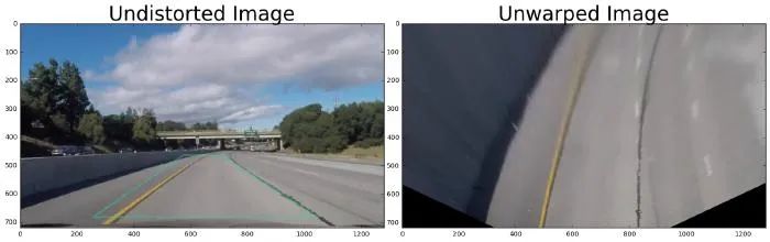未扭曲的图像

这种转换非常简单，我们在屏幕上取四个我们知道的点，然后将它们转换为屏幕的期望位置。让我们使用上图的示例更详细地回顾一下，在图片中，我们看到一个绘制在顶部的绿色形状，这个矩形使用四个源点作为角，它与相机的常规直线道路重叠。矩形围绕图像的中心切割，因为透视是街景通常结束的地方，以让位于天空。现在我们把这些点移到屏幕上我们想要的位置，这就是将绿色区域转换成一个矩形，从 0 到图片的高度，下面是我们将在代码中使用的源点和目标点：

height, width, color = img.shape


src = np.float32([
    [210, height],
    [1110, height],
    [580, 460],
    [700, 460]
])


dst = np.float32([
    [210, height],
    [1110, height],
    [210, 0],
    [1110, 0]
])

src, dst = self._calc_warp_points(img)


if self._M is None:
    self._M = cv2.getPerspectiveTransform(src, dst)
    self._M_inv = cv2.getPerspectiveTransform(dst, src)


return cv2.warpPerspective(img, self._M, (width, height), flags=cv2.INTER_LINEAR)

使用颜色变换、渐变等来创建阈值二值图像。

现在我们已经有了图像，我们需要开始丢弃所有不相关的信息，只保留线条。为此，我们将应用一系列更改，接下来将详细介绍：

转换为灰度

将彩色图像转换为灰度

return cv2.cvtColor(img, cv2.COLOR_RGB2GRAY)

增强图像

通过使用高斯模糊对图像进行平滑，并将原始图像加权到平滑后的图像中，执行一些次要但重要的增强

dst = cv2.GaussianBlur(img, (0, 0), 3)
out = cv2.addWeighted(img, 1.5, dst, -0.5, 0)

使用 Sobel 设置水平梯度的阈值。

计算 X 轴上颜色变化函数的导数，并应用阈值来过滤高强度颜色变化，当我们使用灰度时，这将是边界。

sobel = cv2.Sobel(img, cv2.CV_64F, True, False)
abs_sobel = np.absolute(sobel)
scaled_sobel = np.uint8(255 * abs_sobel / np.max(abs_sobel))


return (scaled_sobel >= 20) & (scaled_sobel <= 220)

使用 Sobel 设置梯度方向阈值，以便仅检测到更接近垂直的边缘。

现在我们计算新阈值的方向导数

# Calculate the x and y gradients
sobel_x = cv2.Sobel(img, cv2.CV_64F, 1, 0, ksize=sobel_kernel)
sobel_y = cv2.Sobel(img, cv2.CV_64F, 0, 1, ksize=sobel_kernel)


# Take the absolute value of the x and y gradients
gradient_direction = np.arctan2(np.absolute(sobel_y), np.absolute(sobel_x))
gradient_direction = np.absolute(gradient_direction)


return (gradient_direction >= np.pi/6) & (gradient_direction <= np.pi*5/6)

接下来，我们将它们组合成一个渐变

# combine the gradient and direction thresholds.
gradient_condition = ((sx_condition == 1) & (dir_condition == 1))

颜色阈值

此过滤器适用于原始图像，我们尝试仅获取那些黄色/白色的像素（如道路线）

r_channel = img[:, :, 0]
g_channel = img[:, :, 1]
return (r_channel > thresh) & (g_channel > thresh)

L层和S层的HSL阈值

对于此任务，有必要更改颜色空间，特别是，我们将使用 HSL 颜色空间，因为它对我们使用的图像具有有趣的特征。

def _hls_condition(self, img, channel, thresh=(220, 255)):
    channels = {
        "h": 0,
        "l": 1,
        "s": 2
    }
    hls = cv2.cvtColor(img, cv2.COLOR_RGB2HLS)


    hls = hls[:, :, channels[channel]]


    return (hls > thresh[0]) & (hls <= thresh[1])

    最后我们将所有这些组合成一个最终图像：

grey = self._to_greyscale(img)
grey = self._enhance(grey)


# apply gradient threshold on the horizontal gradient
sx_condition = self._sobel_gradient_condition(grey, 'x', 20, 220)


# apply gradient direction threshold so that only edges closer to vertical are detected.
dir_condition = self._directional_condition(grey, thresh=(np.pi/6, np.pi*5/6))


# combine the gradient and direction thresholds.
gradient_condition = ((sx_condition == 1) & (dir_condition == 1))


# and color threshold
color_condition = self._color_condition(img, thresh=200)


# now let's take the HSL threshold
l_hls_condition = self._hls_condition(img, channel='l', thresh=(120, 255))
s_hls_condition = self._hls_condition(img, channel='s', thresh=(100, 255))


combined_condition = (l_hls_condition | color_condition) & (s_hls_condition | gradient_condition)
result = np.zeros_like(color_condition)
result[combined_condition] = 1

我们的新图像现在如下图所示：

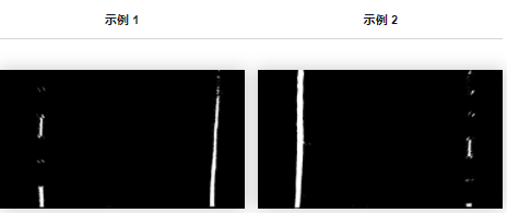
你已经看到那里形成的线条了吗？

检测车道像素并拟合以找到车道边界。

到目前为止，我们已经能够创建一个由只包含车道特征的鸟瞰图组成的图像（至少在大多数情况下，我们仍然有一些噪音）。有了这张新图像，我们现在可以开始进行一些计算，将图像转换为我们可以使用的实际值，例如车道位置和曲率。

让我们首先识别图像上的像素并构建一个表示车道函数的多项式。我们打算怎么做？事实证明，有一个非常好的方法，使用图像下半部分的直方图。下面是直方图的示例：

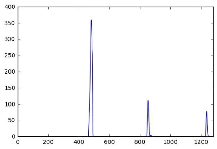直方图

图像上的峰值帮助我们识别车道的左侧和右侧，以下是在代码上构建直方图的方式：

# Take a histogram of the bottom half of the image
histogram = np.sum(binary_warped[binary_warped.shape[0] // 2:, :], axis=0)


# Find the peak of the left and right halves of the histogram
# These will be the starting point for the left and right lines
midpoint = np.int(histogram.shape[0] // 2)
left_x_base = np.argmax(histogram[:midpoint])
right_x_base = np.argmax(histogram[midpoint:]) + midpoint

但我们可能会问，为什么只有下半部分？答案是我们只想关注紧挨着汽车的路段，因为车道可能会形成一条曲线，这会影响我们的直方图。一旦我们找到离汽车更近的车道位置，我们就可以使用移动窗口方法来找到其余车道，如下图所示：

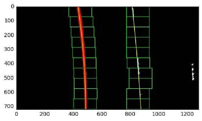移动窗口处理示例

这是它在代码中的样子：

# Choose the number of sliding windows
num_windows = 9
# Set the width of the windows +/- margin
margin = 50
# Set minimum number of pixels found to recenter window
min_pix = 100


# Set height of windows - based on num_windows above and image shape
window_height = np.int(binary_warped.shape[0] // num_windows)


# Current positions to be updated later for each window in nwindows
left_x_current = left_x_base
right_x_current = right_x_base


# Create empty lists to receive left and right lane pixel indices
left_lane_inds = []
right_lane_inds = []


# Step through the windows one by one
for window in range(num_windows):
    # Identify window boundaries in x and y (and right and left)
    win_y_low = binary_warped.shape[0] - (window + 1) * window_height
    win_y_high = binary_warped.shape[0] - window * window_height
    win_x_left_low = left_x_current - margin
    win_x_left_high = left_x_current + margin
    win_x_right_low = right_x_current - margin
    win_x_right_high = right_x_current + margin


    if self._debug:
        # Draw the windows on the visualization image
        cv2.rectangle(out_img, (win_x_left_low, win_y_low),
                      (win_x_left_high, win_y_high), (0, 255, 0), 2)
        cv2.rectangle(out_img, (win_x_right_low, win_y_low),
                      (win_x_right_high, win_y_high), (0, 255, 0), 2)


    # Identify the nonzero pixels in x and y within the window #
    good_left_inds = ((nonzero_y >= win_y_low) & (nonzero_y < win_y_high) &
                      (nonzero_x >= win_x_left_low) & (nonzero_x < win_x_left_high)).nonzero()[0]
    good_right_inds = ((nonzero_y >= win_y_low) & (nonzero_y < win_y_high) &
                       (nonzero_x >= win_x_right_low) & (nonzero_x < win_x_right_high)).nonzero()[0]


    # Append these indices to the lists
    left_lane_inds.append(good_left_inds)
    right_lane_inds.append(good_right_inds)


    # If you found > min_pix pixels, recenter next window on their mean position
    if len(good_left_inds) > min_pix:
        left_x_current = np.int(np.mean(nonzero_x[good_left_inds]))
    if len(good_right_inds) > min_pix:
        right_x_current = np.int(np.mean(nonzero_x[good_right_inds]))


# Concatenate the arrays of indices (previously was a list of lists of pixels)
try:
    left_lane_inds = np.concatenate(left_lane_inds)
    right_lane_inds = np.concatenate(right_lane_inds)
except ValueError:
    # Avoids an error if the above is not implemented fully
    pass

    

这个过程非常紧急，所以在处理视频时，我们可以调整一些事情，因为我们并不总是需要从零开始，之前进行的计算为我们提供了下一个车道的窗口，因此更容易找到. 所有这些都在存储库的最终代码中实现，请随意查看。

一旦我们有了所有的窗口，我们现在可以使用所有确定的点构建多项式，每条线（左和右）将独立计算如下：

left_fit = np.polyfit(left_y, left_x, 2)
right_fit = np.polyfit(right_y, right_x, 2)

数字 2 表示二阶多项式。

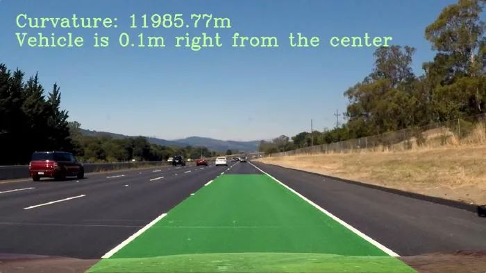
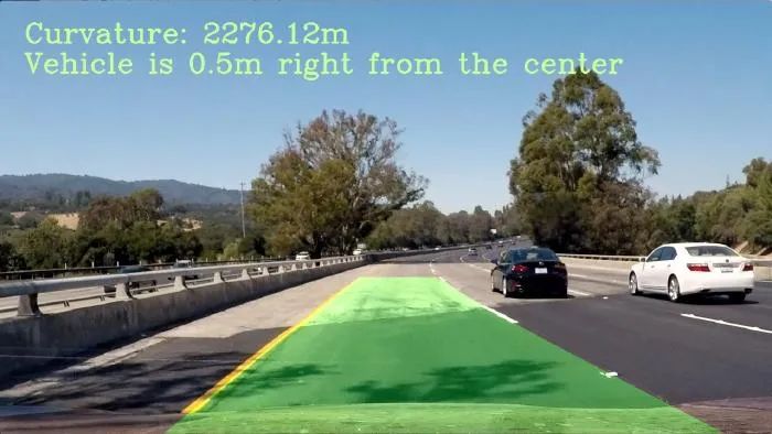
确定车道的曲率和车辆相对于中心的位置。

现在我们知道了线条在图像上的位置，并且我们知道汽车的位置（在相机的中心）我们可以做一些有趣的计算来确定车道的曲率和汽车相对于中心的位置车道的。

车道曲率

车道曲率是一个简单的多项式计算。

fit_cr = np.polyfit(self.all_y * self._ym_per_pix, self.all_x * self._xm_per_pix, 2)
plot_y = np.linspace(0, 720 - 1, 720)
y_eval = np.max(plot_y)


curve = ((1 + (2 * fit_cr[0] * y_eval * self._ym_per_pix + fit_cr[1]) ** 2) ** 1.5) / np.absolute(2 * fit_cr[0])

但是有一个重要的考虑因素，对于这一步，我们不能在像素上工作，我们需要找到一种将像素转换为米的方法，因此我们引入了 2 个变量：_ym_per_pix 和 _xm_per_pix，它们是预定义的值。

self._xm_per_pix = 3.7 / 1280
self._ym_per_pix = 30 / 720

车辆相对于中心的位置

非常简单，计算车道中间的位置，并将其与图像中心进行比较，如下所示

lane_center = (self.left_lane.best_fit[-1] + self.right_lane.best_fit[-1]) / 2
car_center = img.shape[1] / 2
dx = (car_center - lane_center) * self._xm_per_pix

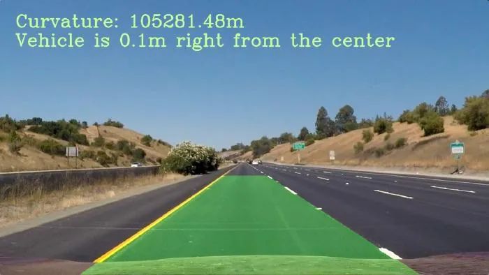
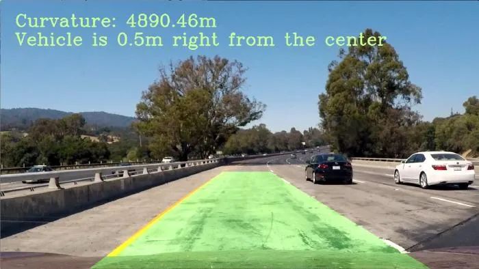
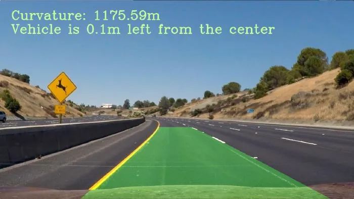
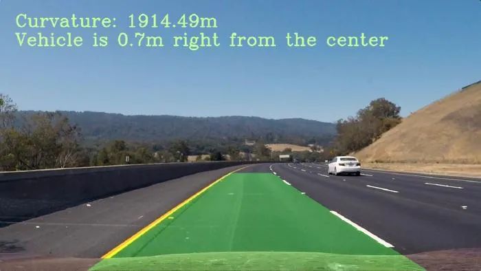
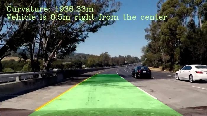
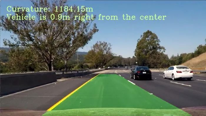
全部完成！

现在我们拥有了所需的所有信息，以及表示车道的多项式，最终结果应如下所示：

Github代码连接：

https://github.com/bajcmartinez/Finding-Car-Lanes-Without-Deep-Learning

下载1：OpenCV-Contrib扩展模块中文版教程

在「小白学视觉」公众号后台回复：扩展模块中文教程，即可下载全网第一份OpenCV扩展模块教程中文版，涵盖扩展模块安装、SFM算法、立体视觉、目标跟踪、生物视觉、超分辨率处理等二十多章内容。

下载2：Python视觉实战项目52讲

在「小白学视觉」公众号后台回复：Python视觉实战项目，即可下载包括图像分割、口罩检测、车道线检测、车辆计数、添加眼线、车牌识别、字符识别、情绪检测、文本内容提取、面部识别等31个视觉实战项目，助力快速学校计算机视觉。

下载3：OpenCV实战项目20讲

在「小白学视觉」公众号后台回复：OpenCV实战项目20讲，即可下载含有20个基于OpenCV实现20个实战项目，实现OpenCV学习进阶。

交流群

欢迎加入公众号读者群一起和同行交流，目前有SLAM、三维视觉、传感器、自动驾驶、计算摄影、检测、分割、识别、医学影像、GAN、算法竞赛等微信群（以后会逐渐细分），请扫描下面微信号加群，备注：”昵称+学校/公司+研究方向“，例如：”张三 + 上海交大 + 视觉SLAM“。请按照格式备注，否则不予通过。添加成功后会根据研究方向邀请进入相关微信群。请勿在群内发送广告，否则会请出群，谢谢理解~