神经网络与深度学习

1、深度学习介绍

深度学习一般是指训练神经网络。
通过给定输入 x 通过神经元得到输出 y 。如：可通过房子的大小来预测房价。
这时可能会得到一个图如下：

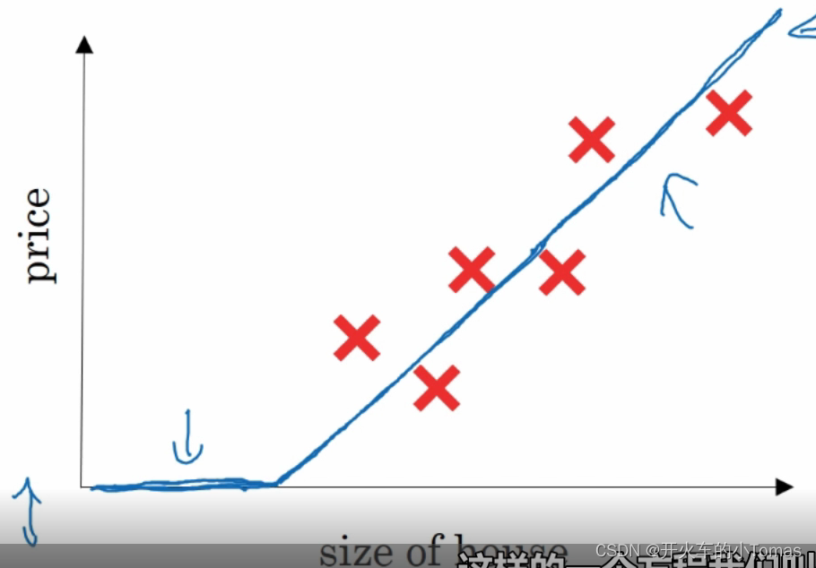
这是一个ReLU函数（Rectified Linerar Unite)，前部分取max(0,y)，后部分取y。

1.1 监督学习和神经网络

1、房价预测，在线广告用的是标准神经网络结构
2、在图像应用中通常使用卷积神经网络（CNN）
3、在序列化数据，如音频文件,语言翻译，通常使用循环神经网络（RNN）
4、如自动驾驶，可能需要更复杂的神经网络。

1.1.1一些概念

神经网络可以用于一些*** 结构化数据和非结构化数据 ***
结构化数据就如数据库中存储的数据
非结构化数据如音频数据和图像数据

2、神经网络基础

一些符号
(x,y) --> x是一个n(x)维的特征向量，y是一个标签取值为0或1。如果有m个训练集，则对应m个(x,y)，以右上标表示是第几个。

2.1、逻辑回归

将一个猫的图片用x表示，然后得到y的值为1。
这个y即图片是猫的概率，若很大则为1，否则0。

约定逻辑回归有一个参数w，和x维度相同。同时还有一个参数b，是一个实数。
此时输出表达式是：，此时是一个线性回归。

但使用这样的式子，并不能保证y的值只有0和1，对于二分类来说不是一个好的算法。

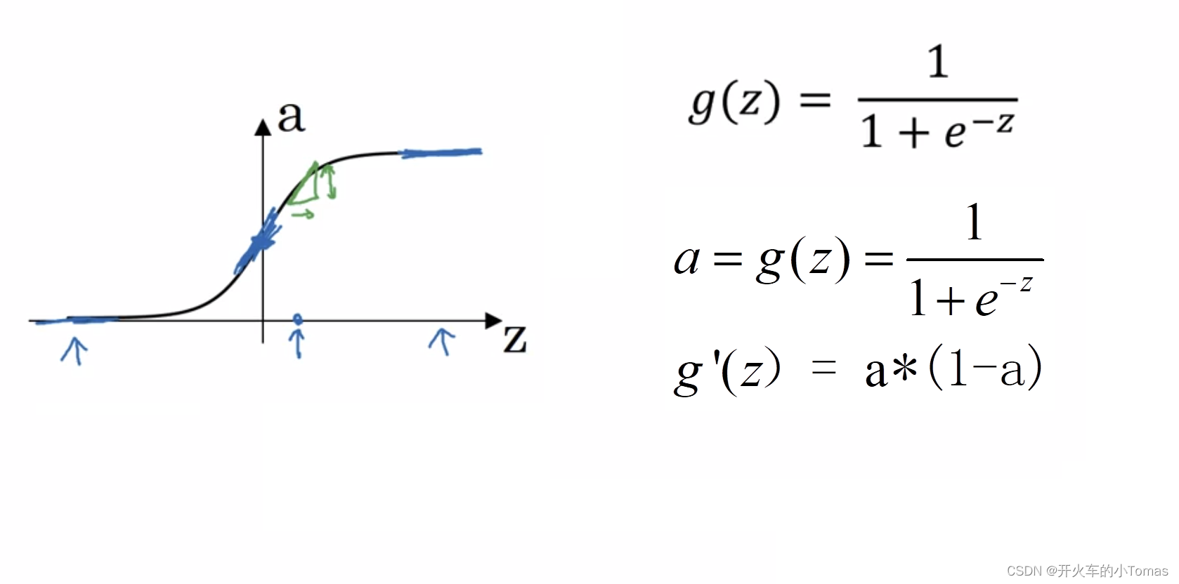
所以有另一种方法，使用函数sigmoid(z)，其中，sigmoid(z)函数则是，它的曲线表达如下图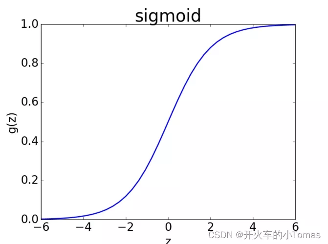：此时，当z很大时，sigmoid函数的值将趋近于1，反之趋近于0。

2.1.1、逻辑回归的损失函数

在训练时，预测值与真实值将会存在偏差，我们当然是要不断调整模型的参数，让偏差值保持最小。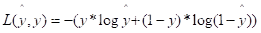这是表示单个样本的优化情况。

如要查看整组的优化情况，使用如下代价函数：

2.1.2、逻辑回归梯度下降

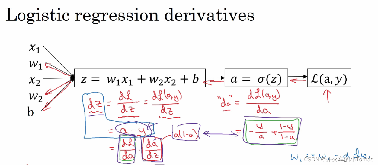
以如上计算图来看：
通过黑色箭头，正向传播将计算出我们的损失函数值。
然后再通过红色箭头进行反向传播，通过链式法则，得到函数值关于变量w和b的梯度值，随后再对这两参数进行更新，如此循环计算出最优解。
其中最右下角蓝色为参数的更新公式，α表示学习率。

2.2、作业点

3、python与向量化

当数据量十分大的时候，使用for循环十分耗时
使用python中numpy库的函数进行向量化计算

import numpy as np 

#以下代码生成a和b，并计算a'*b
#耗费的时间要比 “for i in rang(1000):” 少
a = np.random.rand(1000)
b = np.random.rand(1000)
c = np.dot(a,b)

#   np.sum(a,anis=1,keepdims=true)
#   anis=1表示对矩阵按行求和，0表示按列求和
#   第三个参数保证输出为一个矩阵

python中的广播：
当一个mn的矩阵对一个1n的矩阵进行四则运算，后者将会被复制m次成为一个m*n的矩阵，然后再逐元素进行运算。
广播还有其他特性，这里不另举了。

4、浅层神经网络

神经网络有输入层、隐藏层和输出层，输入层不算入整体的层数计算当中。
如下图所示为一个神经网络：
每一个字母的上标代表属于第几层，下标代表属于第几个神经元
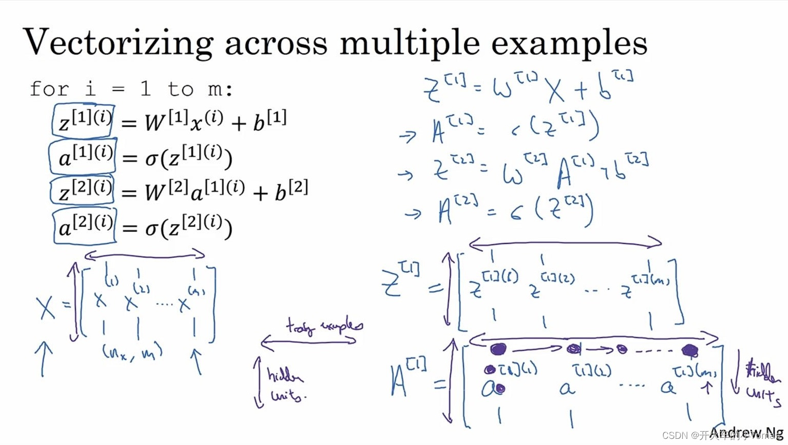
将每个参数向量化后，可以减少循环所带来的时间消耗。

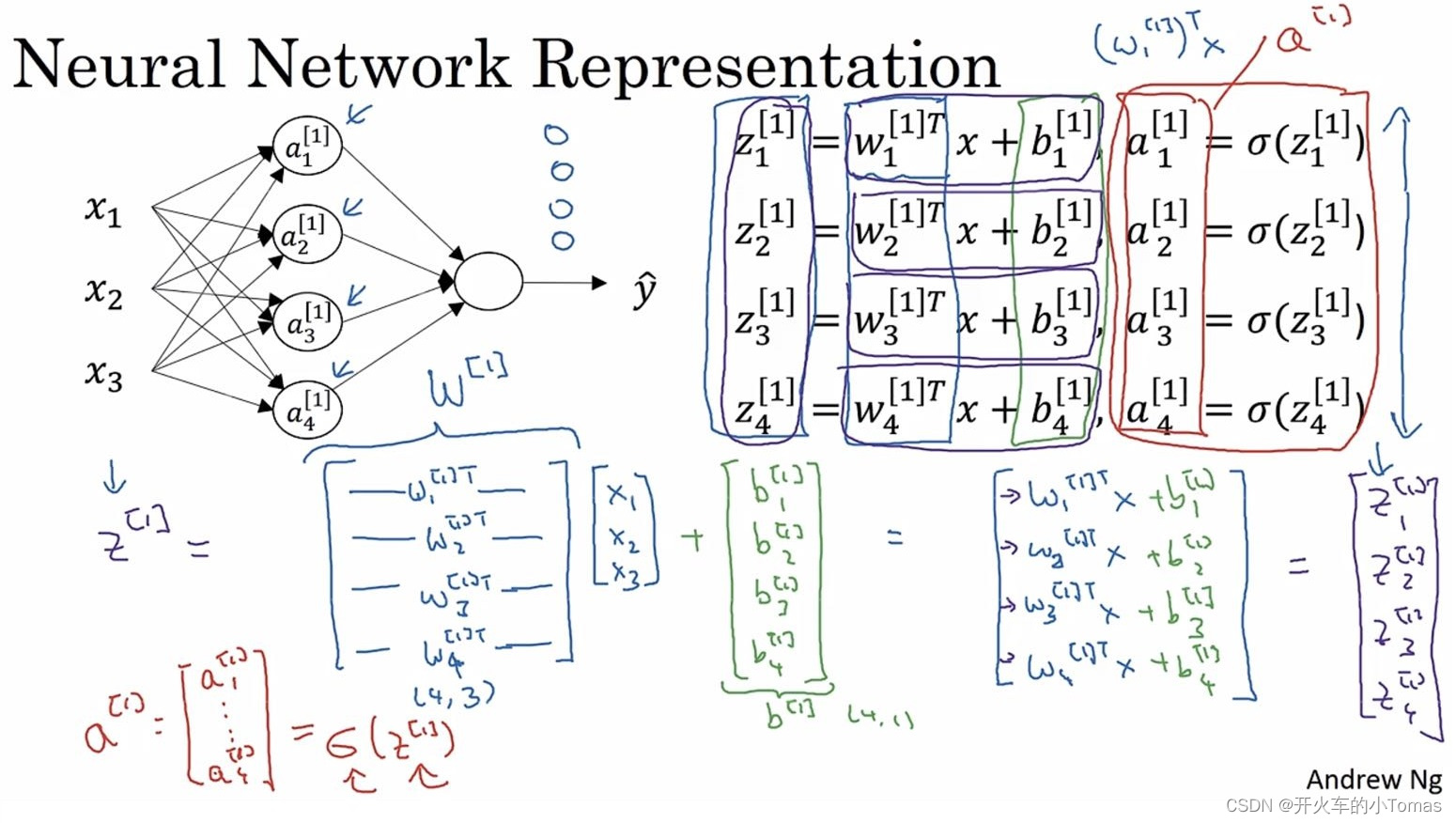
向量化后如下图右下角所示：
从列方向看是按照某一层的不同节点来进行排列，
从行方向看则是按每一层的第某个节点来进行排列

4.1、激活函数

当计算出a的值后，我们可以不选择使用sigmoid作为激活函数，从而选择其他的非线性函数。
sigmoid激活函数一般用于二元分类的输出层，否则不用。

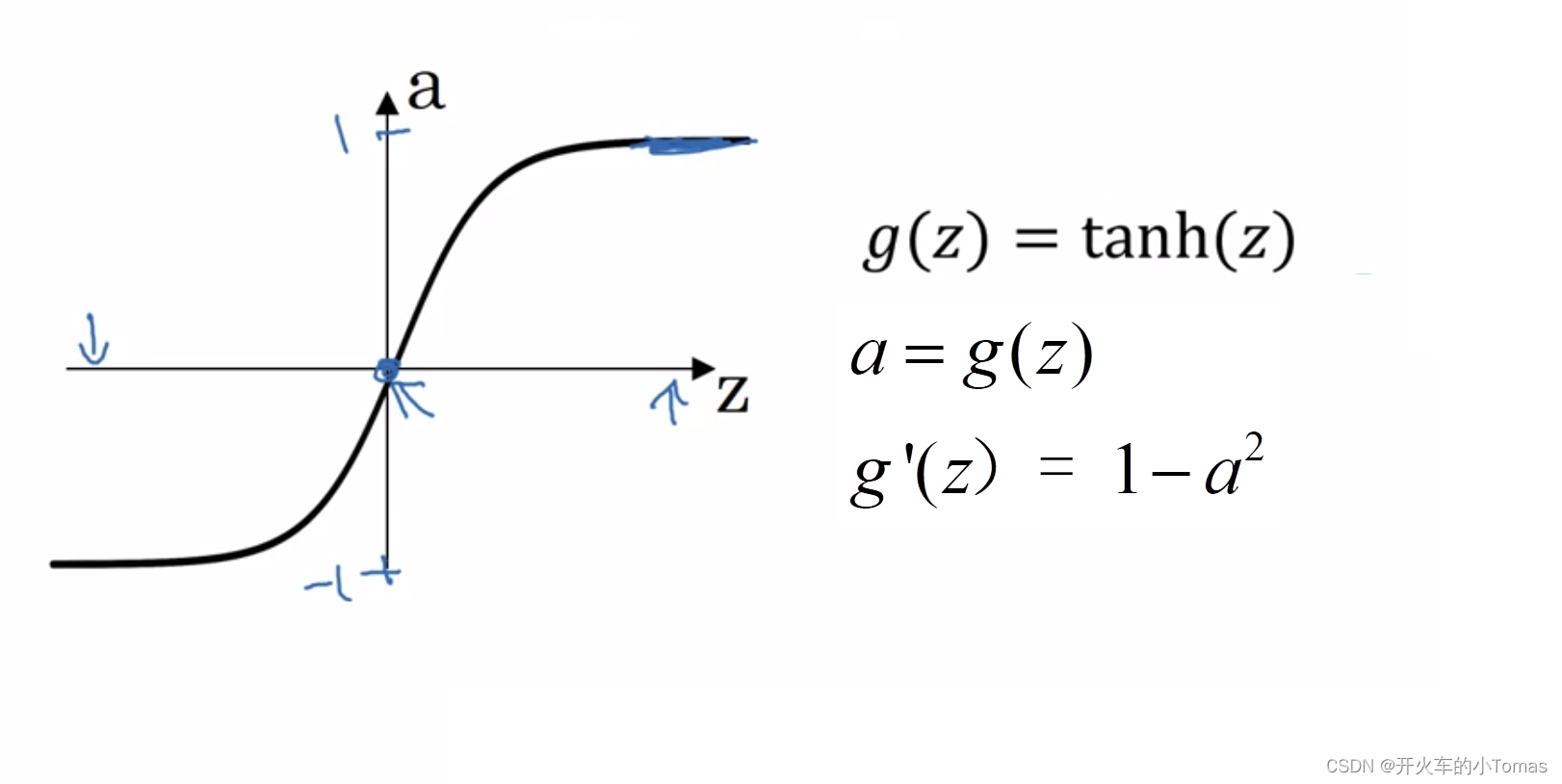
因为tanh函数要比它更好：函数输出介于-1和1之间，激活函数的平均值更接近0，可以让下一层的学习更方便。

另外，上面俩个函数在z很大或很小的时候，函数的斜率接近0，这样使得梯度下降算法会变慢。
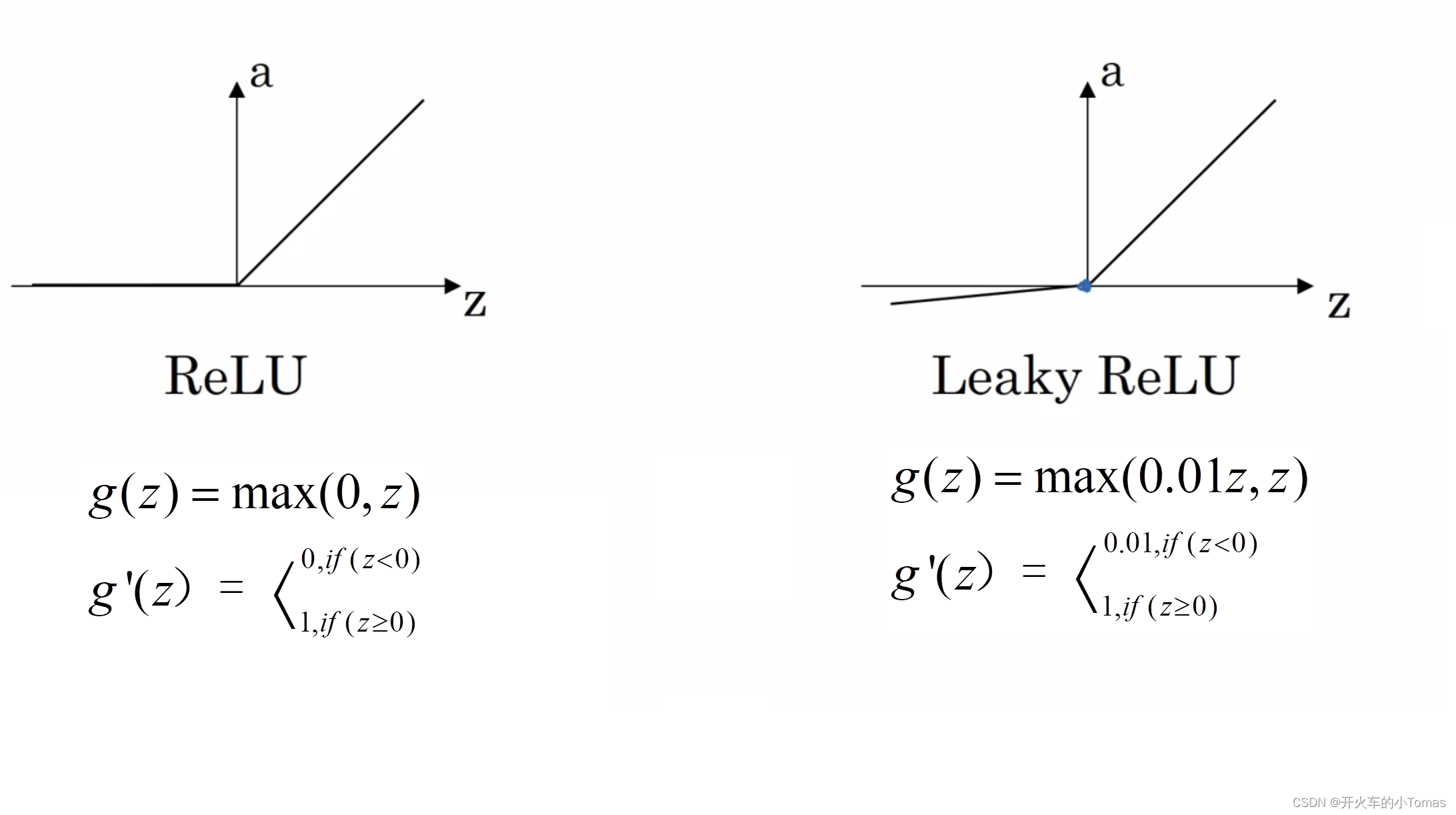
所以一般都会使用ReLu作为默认激活函数，它在z大于0时导数就是1，小于0时导数为0，且在z=0（没有导数定义）时出现概率很低，可以直接给它导数进行赋值

但它仍有缺点，当z为负数时，导数为零。所以提出一个Leaky ReLU，但是使用频率不高。

四个函数图如下所示。

为什么要使用非线性激活函数？
答曰：不使用非线性激活函数，将会使得模型生成与输入线性相关的输出，所以无论使用多少层的神经网络，都只能得到线性的输出，对于结果没有什么作用。

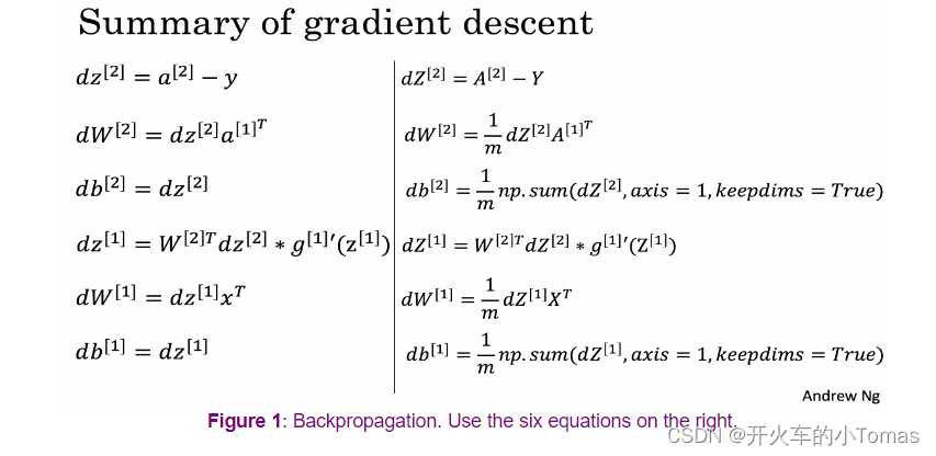
4.2、激活函数的导数

在反向传播中，需要计算导数，那么前一节的四个激活函数的导数分别如下所示：

Sigmoid函数导函数：

tanh函数导函数：

ReLU函数导函数：

5、深层神经网络

5.1、前向传播

通常第一层是 z = wx + b，再将z放入激活函数得到a = g(z)，将a的值传入到下一层，依此类推。
和单隐层神经网络步骤一致，但需要重复几遍

5.2、核对矩阵的维数

一种检查代码是否有误的方法是——核对矩阵的维数
一些参数：

• l —— 表示第 l 层
• n[l] —— 表示第 l 层的节点数
  通常 w[l] 的维度是 ( n[l], n[l-1] )， b[l] 维度则是 （n[l], 1）

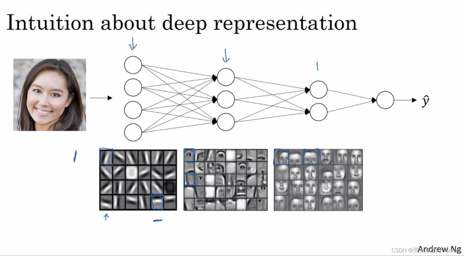
5.3、为什么要深层表示

以人脸识别为例，输入一个脸的图片，在第一层是一个特征探测器（边缘探测器）。
将第一层得到的边缘组合，然后可以组合成面部的不同部分。
最后再把这些部分放在一起就可以识别不同的面部

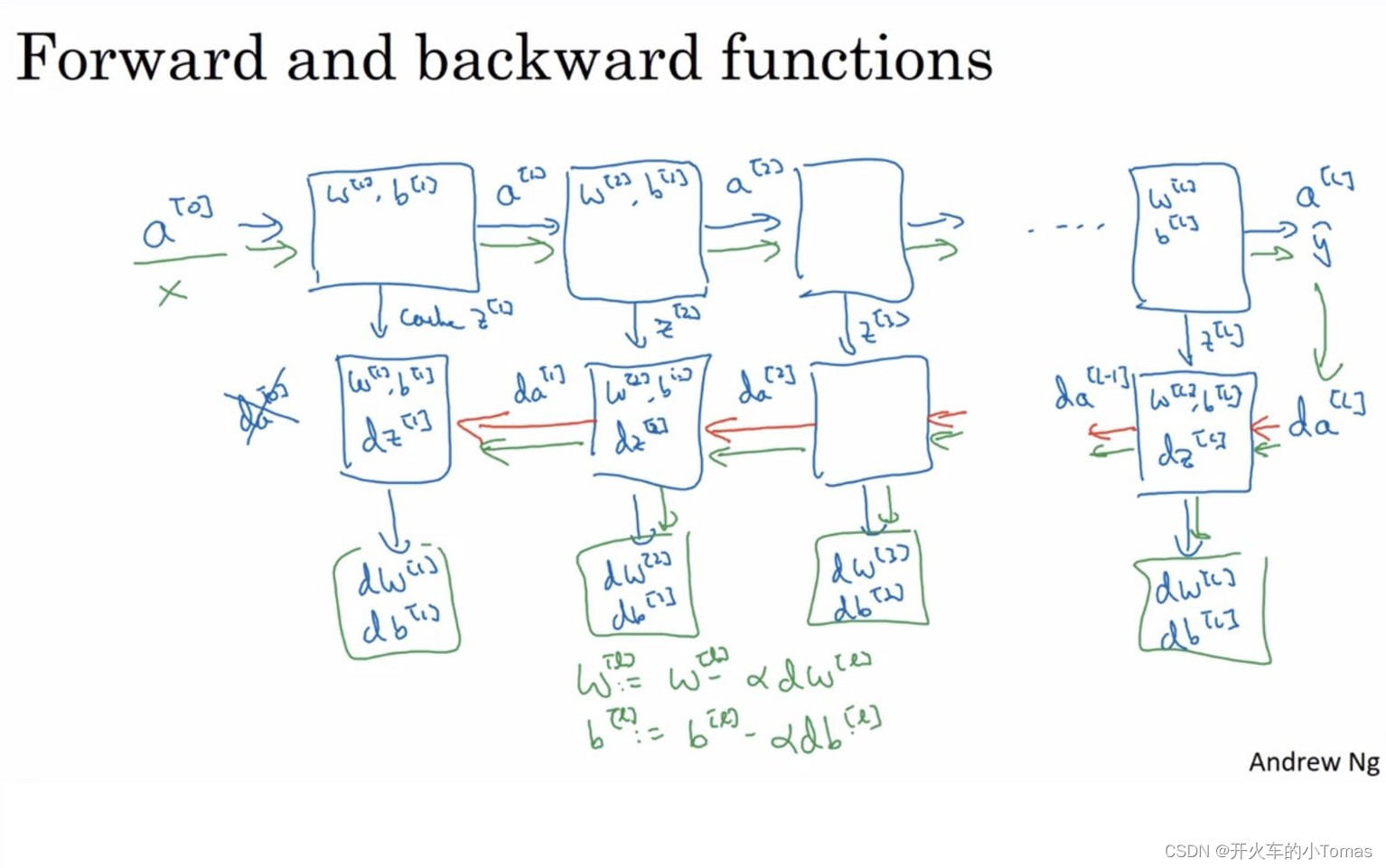
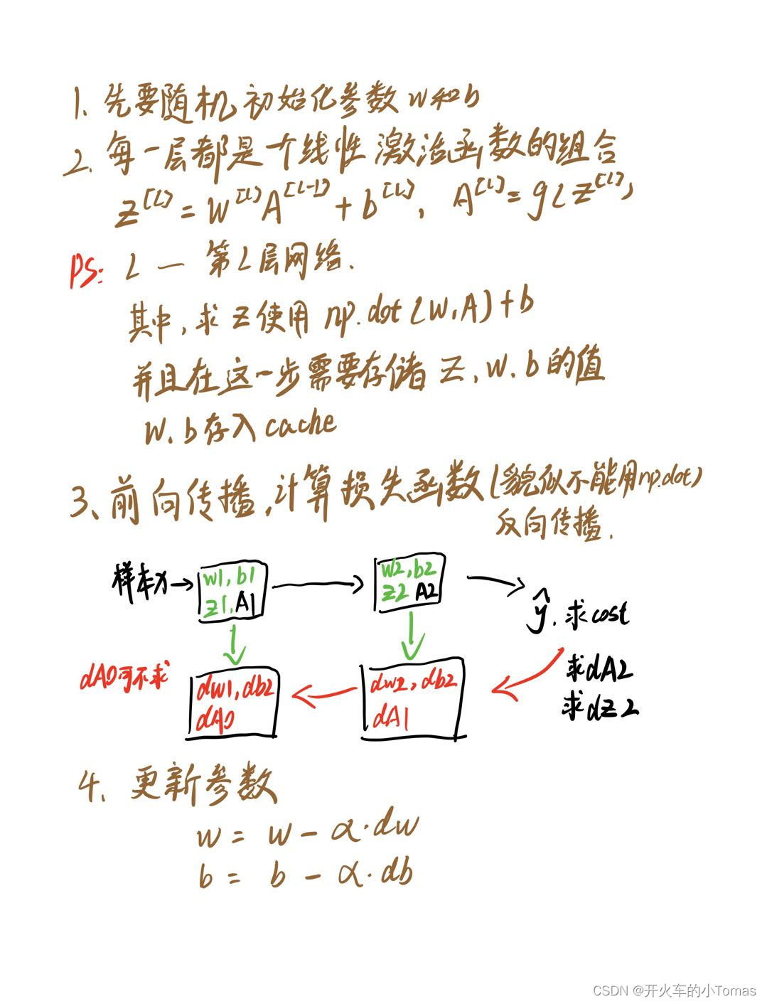
5.4、搭建深层神经网络块

如之前所说，在前向传播每一层开始的时候，我们都能得到w，b参数，以及输入量a。
通过w与b能够计算出这一层z的值，将z存入缓存当中

对于反向传播，有输入da和之前存储的缓存z，以及输出下一层的da与梯度dw，db。通过w和b计算出dz的值。
具体流程如下所示：

5.5、前向传播与反向传播

5.6、 参数与超参数

除了之前所说的w与b作为参数以外，还有如学习率α、梯度下降法循环的次数、隐藏层数L、隐藏单元数n、激活函数选择之类的超参数。
超参数能够决定w和b的值

5.7、 实现自己的神经网络

#导包
import numpy as np #python的科学计算工具
import h5py
import matplotlib.pyplot as plt #python中的画图工具
from testCases import *
from dnn_utils import sigmoid, sigmoid_backward, relu, relu_backward
from public_tests import *

%matplotlib inline
plt.rcParams['figure.figsize'] = (5.0, 4.0) # set default size of plots
plt.rcParams['image.interpolation'] = 'nearest'
plt.rcParams['image.cmap'] = 'gray'

%load_ext autoreload
%autoreload 2

np.random.seed(1)

#这一片代码主要是为下一片深度学习代码所要用到的函数做调用
#具体步骤如下：

#1、初始化参数给2层和L层的神经网络
#1.1、初始化2层的参数
def initialize_parameters(n_x, n_h, n_y):
    """
    Argument:
    n_x -- 输入层的节点数量
    n_h -- 隐藏层的节点数量
    n_y -- 输出层的节点数量
    """  
    np.random.seed(1)
     
     # rand 生成均匀分布的伪随机数。分布在（0~1）之间
     # randn 生成标准正态分布的伪随机数（均值为0，方差为1）
    W1 = np.random.randn(n_h,n_x) * 0.01
    b1 = np.zeros((n_h,1))  # 里面还要打一个括号，用于生成n_h行1列的全零矩阵
    W2 = np.random.randn(n_y,n_h) * 0.01
    b2 = np.zeros((n_y,1))
   
    parameters = {"W1": W1,
                  "b1": b1,
                  "W2": W2,
                  "b2": b2}
 
    return parameters    

#1.2、初始化L层的参数
def initialize_parameters_deep(layer_dims):
    """
    Arguments:
    layer_dims -- 网络中每一层的维度
    """
      
    np.random.seed(3)
    parameters = {}
    L = len(layer_dims) # number of layers in the network

    for l in range(1, L):     
        parameters['W' + str(l)] = np.random.randn(layer_dims[l],layer_dims[l-1]) * 0.01
        parameters['b' + str(l)] = np.zeros((layer_dims[l],1))
        
  
        
        assert(parameters['W' + str(l)].shape == (layer_dims[l], layer_dims[l - 1]))
        assert(parameters['b' + str(l)].shape == (layer_dims[l], 1))
   
    return parameters

Complete the LINEAR part of a layer's forward propagation step (resulting in  𝑍[𝑙] ).
The ACTIVATION function is provided for you (relu/sigmoid)
Combine the previous two steps into a new [LINEAR->ACTIVATION] forward function.
Stack the [LINEAR->RELU] forward function L-1 time (for layers 1 through L-1) and add a [LINEAR->SIGMOID] at the end (for the final layer  𝐿 ). This gives you a new L_model_forward function.

# 2、 实现前向传播模块（需要计算线性和激活函数后的值，已经给出了relu和sigmoid调用函数，L层的神经网络只有最后一层
#	 用sigmoid激活函数，其他层都是用relu函数）
# 2.1、一层前向传播
# 2.1.1、线性传播
def linear_forward(A, W, b):
    """
    Implement the linear part of a layer's forward propagation.

    Arguments:
    A -- activations from previous layer (or input data): (size of previous layer, number of examples)
    W -- weights matrix: numpy array of shape (size of current layer, size of previous layer)
    b -- bias vector, numpy array of shape (size of the current layer, 1)

    """
    
    Z = np.dot(W,A) + b
    cache = (A, W, b)
    
    return Z, cache

# 2..1.2、激活函数的选择
def linear_activation_forward(A_prev, W, b, activation):
    """
    Implement the forward propagation for the LINEAR->ACTIVATION layer

    Arguments:
    A_prev -- 前一层的a函数或者是输入函数: (size of previous layer, number of examples)
    W -- 权重矩阵 (size of current layer, size of previous layer)
    b -- 偏差矩阵, numpy array of shape (size of the current layer, 1)
    activation -- the activation to be used in this layer, stored as a text string: "sigmoid" or "relu"

    Returns:
    A -- the output of the activation function, also called the post-activation value 
    cache -- a python tuple containing "linear_cache" and "activation_cache";
             stored for computing the backward pass efficiently
    """
    
    if activation == "sigmoid":        
        Z, linear_cache = linear_forward(A_prev, W, b)
        A, activation_cache = sigmoid(Z)
    
    elif activation == "relu":
    
        Z, linear_cache = linear_forward(A_prev, W, b)
        A, activation_cache = relu(Z)
          
    # linear_cache 存储的a w b 参数
    # activation_cache 存储的 z 参数
    cache = (linear_cache, activation_cache)

    return A, cache

# 2.2、L层前向传播
def L_model_forward(X, parameters):
    """
    Implement forward propagation for the [LINEAR->RELU]*(L-1)->LINEAR->SIGMOID computation
    
    Arguments:
    X -- data, numpy array of shape (input size, number of examples)
    parameters -- w和b参数的矩阵
    
    Returns:
    AL -- activation value from the output (last) layer
    caches -- list of caches containing:
                every cache of linear_activation_forward() (there are L of them, indexed from 0 to L-1)
    """

    caches = []
    A = X
    L = len(parameters) // 2                  # number of layers in the neural network
    
    # Implement [LINEAR -> RELU]*(L-1). Add "cache" to the "caches" list.
    # The for loop starts at 1 because layer 0 is the input
    for l in range(1, L):
        A_prev = A      
        # 这里caches存储的有 Z 和 W 、 b 的值
        A, cache = linear_activation_forward(A_prev, parameters["W" + str(l)], parameters["b" + str(l)],activation="relu")
        caches.append(cache)
  
    # Implement LINEAR -> SIGMOID. Add "cache" to the "caches" list.
       
    AL, cache = linear_activation_forward(A, parameters["W" + str(L)], parameters["b" + str(L)],activation="sigmoid")
    caches.append(cache)
    
    return AL, caches

# 3、计算代价函数
def compute_cost(AL, Y):
    """
    Arguments:
    AL -- probability vector corresponding to your label predictions, shape (1, number of examples).。。。。预测值
    Y -- true "label" vector (for example: containing 0 if non-cat, 1 if cat), shape (1, number of examples)。。。真实值

    Returns:
    cost -- cross-entropy cost
    """
    
    m = Y.shape[1]

    #用不了np.dot(Y, np.log(AL))，我猜测用不了是因为代价函数计算所使用的不是矩阵,而是对数值进行乘法
    #cost = - np.sum(np.multiply(Y,np.log(AL)) + np.multiply((1-Y),np.log(1-AL)), axis=1 ,keepdims=True) / m
    cost = - np.sum(Y*np.log(AL) + (1-Y)*np.log(1-AL), axis=1 ,keepdims=True) / m
        
    cost = np.squeeze(cost)      # To make sure your cost's shape is what we expect (e.g. this turns [[17]] into 17).
    
    return cost


# 4、实现反向传播模块
# 4.1、 看np,sum函数功能
A = np.array([[1, 2], [3, 4]])
print('axis=1 and keepdims=True')
print(np.sum(A, axis=1, keepdims=True))
print('axis=1 and keepdims=False')![请添加图片描述](https://img-blog.csdnimg.cn/79e0c65b7c8b4b269bb0970813bc9c1a.jpeg)

print(np.sum(A, axis=1, keepdims=False))
print('axis=0 and keepdims=True')
print(np.sum(A, axis=0, keepdims=True))
print('axis=0 and keepdims=False')
print(np.sum(A, axis=0, keepdims=False))
# anis = 1 表示对矩阵按行求和，每一行的和最终构成了一个列向量
# anis = 0 表示按列求和，每一列的求和最终构成了一个行向量
#输出结果如下：
#          axis=1 and keepdims=True
#          [[3]
#           [7]]
#          axis=1 and keepdims=False
#          [3 7]
#          axis=0 and keepdims=True
#          [[4 6]]
#          axis=0 and keepdims=False
#          [4 6]

# 4.2、反向传播的线性部分
def linear_backward(dZ, cache):
    """
    Implement the linear portion of backward propagation for a single layer (layer l)

    Arguments:
    dZ -- Gradient of the cost with respect to the linear output (of current layer l)
    cache -- tuple of values (A_prev, W, b) coming from the forward propagation in the current layer

    Returns:
    dA_prev -- Gradient of the cost with respect to the activation (of the previous layer l-1), same shape as A_prev
    dW -- Gradient of the cost with respect to W (current layer l), same shape as W
    db -- Gradient of the cost with respect to b (current layer l), same shape as b
    """
    A_prev, W, b = cache
    m = A_prev.shape[1]
    
    dW = np.dot(dZ, A_prev.T) / m
    db = np.sum(dZ,axis = 1, keepdims = True) /m
    dA_prev = np.dot(W.T,dZ)
    
    return dA_prev, dW, db

# 4.3、反向线性激活
def linear_activation_backward(dA, cache, activation):
    """
    Implement the backward propagation for the LINEAR->ACTIVATION layer.
    
    Arguments:
    dA -- post-activation gradient for current layer l 
    cache -- tuple of values (linear_cache, activation_cache) we store for computing backward propagation efficiently
    activation -- the activation to be used in this layer, stored as a text string: "sigmoid" or "relu"
    
    Returns:
    dA_prev -- Gradient of the cost with respect to the activation (of the previous layer l-1), same shape as A_prev
    dW -- Gradient of the cost with respect to W (current layer l), same shape as W
    db -- Gradient of the cost with respect to b (current layer l), same shape as b
    """
    linear_cache, activation_cache = cache
    
    if activation == "relu":
        dZ =  relu_backward(dA, activation_cache)
        dA_prev, dW, db = linear_backward(dZ, linear_cache)
        
    elif activation == "sigmoid":   
        dZ =  sigmoid_backward(dA, activation_cache)
        dA_prev, dW, db = linear_backward(dZ, linear_cache)
        
    return dA_prev, dW, db

# 4.4、L层反向传播模型
def L_model_backward(AL, Y, caches):
    """
    Implement the backward propagation for the [LINEAR->RELU] * (L-1) -> LINEAR -> SIGMOID group
    
    Arguments:
    AL -- probability vector, output of the forward propagation (L_model_forward())
    Y -- true "label" vector (containing 0 if non-cat, 1 if cat)
    caches -- list of caches containing:
                every cache of linear_activation_forward() with "relu" (it's caches[l], for l in range(L-1) i.e l = 0...L-2)
                the cache of linear_activation_forward() with "sigmoid" (it's caches[L-1])
    
    Returns:
    grads -- A dictionary with the gradients
             grads["dA" + str(l)] = ... 
             grads["dW" + str(l)] = ...
             grads["db" + str(l)] = ... 
    """
    grads = {}
    L = len(caches) # the number of layers
    m = AL.shape[1]
    Y = Y.reshape(AL.shape) # after this line, Y is the same shape as AL
    
    #求最后一层的da
    dAL =  - (np.divide(Y, AL) - np.divide(1 - Y, 1 - AL))
    
    # Lth layer (SIGMOID -> LINEAR) gradients. Inputs: "dAL, current_cache". Outputs: "grads["dAL-1"], grads["dWL"], grads["dbL"]
    # 对应sigmoid激活函数的反向求导
    cache=caches[-1]
    grads["dA"+str(L-1)],grads["dW"+str(L)],grads["db"+str(L)]=linear_activation_backward(dAL,cache,activation="sigmoid")

    
    # Loop from l=L-2 to l=0 
    # 对应前L-1层的relu激活函数反向推导
    for l in reversed(range(L-1)):
        cache=caches[l]
        dA_prev, dW, db = linear_activation_backward(grads["dA" + str(l + 1)], cache, activation = "relu")
        grads["dA" + str(l)]=dA_prev
        grads["dW" + str(l + 1)]=dW
        grads["db" + str(l + 1)]=db

    return grads

# 4.5、更新参数
def update_parameters(params, grads, learning_rate):
    """
    Update parameters using gradient descent
    
    Arguments:
    params -- python dictionary containing your parameters 
    grads -- python dictionary containing your gradients, output of L_model_backward
    
    Returns:
    parameters -- python dictionary containing your updated parameters 
                  parameters["W" + str(l)] = ... 
                  parameters["b" + str(l)] = ...
    """
    parameters = params.copy()
    L = len(parameters) // 2 # number of layers in the neural network

    # Update rule for each parameter. Use a for loop.
    #(≈ 2 lines of code)
    for l in range(L):
        parameters["W" + str(l+1)] = parameters["W" + str(l+1)] - learning_rate*grads["dW"+str(l+1)]
        parameters["b" + str(l+1)] = parameters["b" + str(l+1)] - learning_rate*grads["db"+str(l+1)]
    return parameters

Note:

For every forward function, there is a corresponding backward function. This is why at every step of your forward module you will be storing some values in a cache. These cached values are useful for computing gradients.

In the backpropagation module, you can then use the cache to calculate the gradients. Don't worry, this assignment will show you exactly how to carry out each of these steps!

神经网络判断图片是否为猫，先导包

import time
import numpy as np
import h5py
import matplotlib.pyplot as plt
import scipy
from PIL import Image
from scipy import ndimage
from dnn_app_utils_v3 import *
from public_tests import *

%matplotlib inline
plt.rcParams['figure.figsize'] = (5.0, 4.0) # set default size of plots
plt.rcParams['image.interpolation'] = 'nearest'
plt.rcParams['image.cmap'] = 'gray'

%load_ext autoreload
%autoreload 2

np.random.seed(1)

获取数据集

train_x_orig, train_y, test_x_orig, test_y, classes = load_data()
m_train = train_x_orig.shape[0]
num_px = train_x_orig.shape[1]
m_test = test_x_orig.shape[0]

print ("Number of training examples: " + str(m_train))
print ("Number of testing examples: " + str(m_test))
print ("Each image is of size: (" + str(num_px) + ", " + str(num_px) + ", 3)")
print ("train_x_orig shape: " + str(train_x_orig.shape))
print ("train_y shape: " + str(train_y.shape))
print ("test_x_orig shape: " + str(test_x_orig.shape))
print ("test_y shape: " + str(test_y.shape))

结果如下：

Number of training examples: 209
Number of testing examples: 50
Each image is of size: (64, 64, 3)
train_x_orig shape: (209, 64, 64, 3)
train_y shape: (1, 209)
test_x_orig shape: (50, 64, 64, 3)
test_y shape: (1, 50)

两层的神经网络如下：

### CONSTANTS DEFINING THE MODEL ####
n_x = 12288     # num_px * num_px * 3
n_h = 7
n_y = 1
layers_dims = (n_x, n_h, n_y)
learning_rate = 0.0075

# 在此处定义模型
def two_layer_model(X, Y, layers_dims, learning_rate = 0.0075, num_iterations = 3000, print_cost=False):
    """
    Implements a two-layer neural network: LINEAR->RELU->LINEAR->SIGMOID.
    
    Arguments:
    X -- input data, of shape (n_x, number of examples)
    Y -- true "label" vector (containing 1 if cat, 0 if non-cat), of shape (1, number of examples)
    layers_dims -- dimensions of the layers (n_x, n_h, n_y) 每一层的维度
    num_iterations -- number of iterations of the optimization loop
    learning_rate -- learning rate of the gradient descent update rule
    print_cost -- If set to True, this will print the cost every 100 iterations 
    
    Returns:
    parameters -- a dictionary containing W1, W2, b1, and b2
    """
    
    np.random.seed(1)
    grads = {}
    costs = []                              # to keep track of the cost
    m = X.shape[1]                           # number of examples
    (n_x, n_h, n_y) = layers_dims
    
    #初始化参数
    parameters = initialize_parameters(n_x, n_h, n_y)
    
    # Get W1, b1, W2 and b2 from the dictionary parameters.
    W1 = parameters["W1"]
    b1 = parameters["b1"]
    W2 = parameters["W2"]
    b2 = parameters["b2"]
    
    # Loop (gradient descent)
    for i in range(0, num_iterations):

        # Forward propagation: LINEAR -> RELU -> LINEAR -> SIGMOID. Inputs: "X, W1, b1, W2, b2". Output: "A1, cache1, A2, cache2".
        #(≈ 2 lines of code)
        # A1, cache1 = ...
        # A2, cache2 = ...
        # YOUR CODE STARTS HERE
        
        A1, cache1 = linear_activation_forward(X,W1,b1,"relu")
        A2, cache2 = linear_activation_forward(A1,W2,b2,"sigmoid")
        
        # YOUR CODE ENDS HERE
        
        # Compute cost
        #(≈ 1 line of code)
        # cost = ...
        # YOUR CODE STARTS HERE
        
        cost = compute_cost(A2,Y)
        
        # YOUR CODE ENDS HERE
        
        # Initializing backward propagation
        dA2 = - (np.divide(Y, A2) - np.divide(1 - Y, 1 - A2))
        
        # Backward propagation. Inputs: "dA2, cache2, cache1". Outputs: "dA1, dW2, db2; also dA0 (not used), dW1, db1".
        #(≈ 2 lines of code)
        # dA1, dW2, db2 = ...
        # dA0, dW1, db1 = ...
        # YOUR CODE STARTS HERE
        
        dA1, dW2, db2 = linear_activation_backward(dA2, cache2, "sigmoid")
        dA0, dW1, db1 = linear_activation_backward(dA1, cache1, "relu")
        
        # YOUR CODE ENDS HERE
        
        # Set grads['dWl'] to dW1, grads['db1'] to db1, grads['dW2'] to dW2, grads['db2'] to db2
        grads['dW1'] = dW1
        grads['db1'] = db1
        grads['dW2'] = dW2
        grads['db2'] = db2
        
        # Update parameters.
        #(approx. 1 line of code)
        # parameters = ...
        # YOUR CODE STARTS HERE
        
        parameters = update_parameters(parameters, grads, learning_rate)
        
        # YOUR CODE ENDS HERE

        # Retrieve W1, b1, W2, b2 from parameters
        W1 = parameters["W1"]
        b1 = parameters["b1"]
        W2 = parameters["W2"]
        b2 = parameters["b2"]
        
        # Print the cost every 100 iterations
        if print_cost and i % 100 == 0 or i == num_iterations - 1:
            print("Cost after iteration {}: {}".format(i, np.squeeze(cost)))
        if i % 100 == 0 or i == num_iterations:
            costs.append(cost)

    return parameters, costs

def plot_costs(costs, learning_rate=0.0075):
    plt.plot(np.squeeze(costs))
    plt.ylabel('cost')
    plt.xlabel('iterations (per hundreds)')
    plt.title("Learning rate =" + str(learning_rate))
    plt.show()

L层的神经网络如下（使用的层数为4）：

### CONSTANTS ###
layers_dims = [12288, 20, 7, 5, 1] #  4-layer model

# GRADED FUNCTION: L_layer_model

def L_layer_model(X, Y, layers_dims, learning_rate = 0.0075, num_iterations = 3000, print_cost=False):
    """
    Implements a L-layer neural network: [LINEAR->RELU]*(L-1)->LINEAR->SIGMOID.
    
    Arguments:
    X -- data, numpy array of shape (num_px * num_px * 3, number of examples)
    Y -- true "label" vector (containing 0 if cat, 1 if non-cat), of shape (1, number of examples)
    layers_dims -- list containing the input size and each layer size, of length (number of layers + 1).
    learning_rate -- learning rate of the gradient descent update rule
    num_iterations -- number of iterations of the optimization loop
    print_cost -- if True, it prints the cost every 100 steps
    
    Returns:
    parameters -- parameters learnt by the model. They can then be used to predict.
    """

    np.random.seed(1)
    costs = []                         # keep track of cost
    
    # Parameters initialization.
    #(≈ 1 line of code)
    # parameters = ...
    # YOUR CODE STARTS HERE
    
    parameters = initialize_parameters_deep(layers_dims)
    
    # YOUR CODE ENDS HERE
    
    # Loop (gradient descent)
    for i in range(0, num_iterations):

        # Forward propagation: [LINEAR -> RELU]*(L-1) -> LINEAR -> SIGMOID.
        #(≈ 1 line of code)
        # AL, caches = ...
        # YOUR CODE STARTS HERE
        
        AL, caches = L_model_forward(X, parameters)
        
        # YOUR CODE ENDS HERE
        
        # Compute cost.
        #(≈ 1 line of code)
        # cost = ...
        # YOUR CODE STARTS HERE
        
        cost = compute_cost(AL, Y)
        
        # YOUR CODE ENDS HERE
    
        # Backward propagation.
        #(≈ 1 line of code)
        # grads = ...    
        # YOUR CODE STARTS HERE
        
        grads = L_model_backward(AL, Y, caches)
        
        # YOUR CODE ENDS HERE
 
        # Update parameters.
        #(≈ 1 line of code)
        # parameters = ...
        # YOUR CODE STARTS HERE
        
        parameters = update_parameters(parameters, grads, learning_rate)
        
        # YOUR CODE ENDS HERE
                
        # Print the cost every 100 iterations
        if print_cost and i % 100 == 0 or i == num_iterations - 1:
            print("Cost after iteration {}: {}".format(i, np.squeeze(cost)))
        if i % 100 == 0 or i == num_iterations:
            costs.append(cost)
    
    return parameters, costs

6、总结

一、建立一个神经网络的方法步骤通常如下：

1. 定义好神经网络的结构，如输入单元，隐藏单元等。
2. 初始化模型的参数，如w进行随机初始化（若初始化全为0，则不会有变化发生）
3. 循环：

   • 实现前向传播

   • 计算损失函数

   • 实现后向传播计算梯度在这里插入图片描述

   • 更新参数
     随后可将如上步骤集成进一个函数，该模型函数就可以训练参数。

二、 一些numpy函数
np.multiply函数：数组与矩阵对应位置相乘
np.dot函数：

• 1、秩为1的数组，对应位置相乘然后再相加。
• 2、秩不为1的二维数组，执行矩阵乘法运算

三、反向传播总结

7、还有一件事（自己没太弄清的点）

7.1、一套训练的流程是怎么样的？

7.2、np.dot、np.multiply、*号之间的用法。

两个向量使用dot则得到两个向量的内积

两个矩阵使用dot则等同于矩阵乘法

multiply就是对应位置的元素相乘，*与multiply相同

参考于：https://blog.csdn.net/bitcarmanlee/article/details/120886711