02-FeatureScaling归一化

数据归一化，将所有的数据映射到同一尺度

最值归一化：把所有数据映射到0-1之间

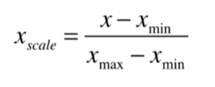
适用于分布有明显边界的情况,有最大值最小值

均值方差归一化：把所有数据归一到均值为0方差为1的分布中

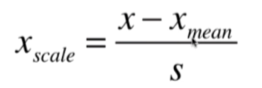
数据有没有明显边界都可以，不能保证数据在0-1之间，可能存在极端数据值

使用均值方差归一化进行乳腺癌数据集的实战

import numpy as np
from sklearn import datasets
import matplotlib.pyplot as plt
%matplotlib inline

"""加载乳腺癌数据集"""
breast_cancer=datasets.load_breast_cancer()

breast_cancer.keys()

dict_keys(['data', 'target', 'frame', 'target_names', 'DESCR', 'feature_names', 'filename'])

"""查看数据描述"""
"""可以看到这个数据集特征的最值差别是比较大的"""
print(breast_cancer.DESCR)

.. _breast_cancer_dataset:

Breast cancer wisconsin (diagnostic) dataset
--------------------------------------------

**Data Set Characteristics:**

    :Number of Instances: 569

    :Number of Attributes: 30 numeric, predictive attributes and the class

    :Attribute Information:
        - radius (mean of distances from center to points on the perimeter)
        - texture (standard deviation of gray-scale values)
        - perimeter
        - area
        - smoothness (local variation in radius lengths)
        - compactness (perimeter^2 / area - 1.0)
        - concavity (severity of concave portions of the contour)
        - concave points (number of concave portions of the contour)
        - symmetry
        - fractal dimension ("coastline approximation" - 1)

        The mean, standard error, and "worst" or largest (mean of the three
        worst/largest values) of these features were computed for each image,
        resulting in 30 features.  For instance, field 0 is Mean Radius, field
        10 is Radius SE, field 20 is Worst Radius.

        - class:
                - WDBC-Malignant
                - WDBC-Benign

    :Summary Statistics:

    ===================================== ====== ======
                                           Min    Max
    ===================================== ====== ======
    radius (mean):                        6.981  28.11
    texture (mean):                       9.71   39.28
    perimeter (mean):                     43.79  188.5
    area (mean):                          143.5  2501.0
    smoothness (mean):                    0.053  0.163
    compactness (mean):                   0.019  0.345
    concavity (mean):                     0.0    0.427
    concave points (mean):                0.0    0.201
    symmetry (mean):                      0.106  0.304
    fractal dimension (mean):             0.05   0.097
    radius (standard error):              0.112  2.873
    texture (standard error):             0.36   4.885
    perimeter (standard error):           0.757  21.98
    area (standard error):                6.802  542.2
    smoothness (standard error):          0.002  0.031
    compactness (standard error):         0.002  0.135
    concavity (standard error):           0.0    0.396
    concave points (standard error):      0.0    0.053
    symmetry (standard error):            0.008  0.079
    fractal dimension (standard error):   0.001  0.03
    radius (worst):                       7.93   36.04
    texture (worst):                      12.02  49.54
    perimeter (worst):                    50.41  251.2
    area (worst):                         185.2  4254.0
    smoothness (worst):                   0.071  0.223
    compactness (worst):                  0.027  1.058
    concavity (worst):                    0.0    1.252
    concave points (worst):               0.0    0.291
    symmetry (worst):                     0.156  0.664
    fractal dimension (worst):            0.055  0.208
    ===================================== ====== ======

    :Missing Attribute Values: None

    :Class Distribution: 212 - Malignant, 357 - Benign

    :Creator:  Dr. William H. Wolberg, W. Nick Street, Olvi L. Mangasarian

    :Donor: Nick Street

    :Date: November, 1995

This is a copy of UCI ML Breast Cancer Wisconsin (Diagnostic) datasets.
https://goo.gl/U2Uwz2

Features are computed from a digitized image of a fine needle
aspirate (FNA) of a breast mass.  They describe
characteristics of the cell nuclei present in the image.

Separating plane described above was obtained using
Multisurface Method-Tree (MSM-T) [K. P. Bennett, "Decision Tree
Construction Via Linear Programming." Proceedings of the 4th
Midwest Artificial Intelligence and Cognitive Science Society,
pp. 97-101, 1992], a classification method which uses linear
programming to construct a decision tree.  Relevant features
were selected using an exhaustive search in the space of 1-4
features and 1-3 separating planes.

The actual linear program used to obtain the separating plane
in the 3-dimensional space is that described in:
[K. P. Bennett and O. L. Mangasarian: "Robust Linear
Programming Discrimination of Two Linearly Inseparable Sets",
Optimization Methods and Software 1, 1992, 23-34].

This database is also available through the UW CS ftp server:

ftp ftp.cs.wisc.edu
cd math-prog/cpo-dataset/machine-learn/WDBC/

.. topic:: References

   - W.N. Street, W.H. Wolberg and O.L. Mangasarian. Nuclear feature extraction 
     for breast tumor diagnosis. IS&T/SPIE 1993 International Symposium on 
     Electronic Imaging: Science and Technology, volume 1905, pages 861-870,
     San Jose, CA, 1993.
   - O.L. Mangasarian, W.N. Street and W.H. Wolberg. Breast cancer diagnosis and 
     prognosis via linear programming. Operations Research, 43(4), pages 570-577, 
     July-August 1995.
   - W.H. Wolberg, W.N. Street, and O.L. Mangasarian. Machine learning techniques
     to diagnose breast cancer from fine-needle aspirates. Cancer Letters 77 (1994) 
     163-171.

all_data=breast_cancer.data
all_label=breast_cancer.target
print('all data shape:{}, all label shape:{}'.format(all_data.shape,all_label.shape))

all data shape:(569, 30), all label shape:(569,)

"""可以看到这个数据集顺序本身应该就是打乱的"""
print(all_label)

[0 0 0 0 0 0 0 0 0 0 0 0 0 0 0 0 0 0 0 1 1 1 0 0 0 0 0 0 0 0 0 0 0 0 0 0 0
 1 0 0 0 0 0 0 0 0 1 0 1 1 1 1 1 0 0 1 0 0 1 1 1 1 0 1 0 0 1 1 1 1 0 1 0 0
 1 0 1 0 0 1 1 1 0 0 1 0 0 0 1 1 1 0 1 1 0 0 1 1 1 0 0 1 1 1 1 0 1 1 0 1 1
 1 1 1 1 1 1 0 0 0 1 0 0 1 1 1 0 0 1 0 1 0 0 1 0 0 1 1 0 1 1 0 1 1 1 1 0 1
 1 1 1 1 1 1 1 1 0 1 1 1 1 0 0 1 0 1 1 0 0 1 1 0 0 1 1 1 1 0 1 1 0 0 0 1 0
 1 0 1 1 1 0 1 1 0 0 1 0 0 0 0 1 0 0 0 1 0 1 0 1 1 0 1 0 0 0 0 1 1 0 0 1 1
 1 0 1 1 1 1 1 0 0 1 1 0 1 1 0 0 1 0 1 1 1 1 0 1 1 1 1 1 0 1 0 0 0 0 0 0 0
 0 0 0 0 0 0 0 1 1 1 1 1 1 0 1 0 1 1 0 1 1 0 1 0 0 1 1 1 1 1 1 1 1 1 1 1 1
 1 0 1 1 0 1 0 1 1 1 1 1 1 1 1 1 1 1 1 1 1 0 1 1 1 0 1 0 1 1 1 1 0 0 0 1 1
 1 1 0 1 0 1 0 1 1 1 0 1 1 1 1 1 1 1 0 0 0 1 1 1 1 1 1 1 1 1 1 1 0 0 1 0 0
 0 1 0 0 1 1 1 1 1 0 1 1 1 1 1 0 1 1 1 0 1 1 0 0 1 1 1 1 1 1 0 1 1 1 1 1 1
 1 0 1 1 1 1 1 0 1 1 0 1 1 1 1 1 1 1 1 1 1 1 1 0 1 0 0 1 0 1 1 1 1 1 0 1 1
 0 1 0 1 1 0 1 0 1 1 1 1 1 1 1 1 0 0 1 1 1 1 1 1 0 1 1 1 1 1 1 1 1 1 1 0 1
 1 1 1 1 1 1 0 1 0 1 1 0 1 1 1 1 1 0 0 1 0 1 0 1 1 1 1 1 0 1 1 0 1 0 1 0 0
 1 1 1 0 1 1 1 1 1 1 1 1 1 1 1 0 1 0 0 1 1 1 1 1 1 1 1 1 1 1 1 1 1 1 1 1 1
 1 1 1 1 1 1 1 0 0 0 0 0 0 1]

"""数据划分"""
test_size=int(len(all_label)*0.3)
train_data,test_data=all_data[test_size:],all_data[:test_size]
train_label,test_label=all_label[test_size:],all_label[:test_size]

print('train data shape:{}, test data shape:{}'.format(train_data.shape,test_data.shape))

train data shape:(399, 30), test data shape:(170, 30)

"""比较使用归一化对kNN算法的提升"""
from sklearn.model_selection import GridSearchCV
from sklearn.neighbors import KNeighborsClassifier
knn_clf=KNeighborsClassifier()
param_grid=[
    {
        'weights':['uniform'],   #不考虑权重
        'n_neighbors':[k for k in range(1,20)],
    },
    {
        'weights':['distance'], #考虑权重
        'n_neighbors':[k for k in range(1,20)],
        'p':[p for p in range(1,6)]
    },
]

"""未使用归一化的kNN算法网格搜索"""
knn_clf_sg=GridSearchCV(knn_clf,param_grid=param_grid)
knn_clf_sg.fit(train_data,train_label)

GridSearchCV(estimator=KNeighborsClassifier(),
             param_grid=[{'n_neighbors': [1, 2, 3, 4, 5, 6, 7, 8, 9, 10, 11, 12,
                                          13, 14, 15, 16, 17, 18, 19],
                          'weights': ['uniform']},
                         {'n_neighbors': [1, 2, 3, 4, 5, 6, 7, 8, 9, 10, 11, 12,
                                          13, 14, 15, 16, 17, 18, 19],
                          'p': [1, 2, 3, 4, 5], 'weights': ['distance']}])

knn_clf_sg.best_score_

0.9599683544303798

knn_clf_sg.best_params_

{'n_neighbors': 7, 'p': 1, 'weights': 'distance'}

knn_clf_sg.best_estimator_.score(test_data,test_label)

0.8647058823529412

"""对数据进行归一化"""
"""注意要用训练数据进行归一化的均值和方差对测试数据也进行归一化"""
from sklearn.preprocessing import StandardScaler
standardScaler=StandardScaler()
standardScaler.fit(train_data)  #此时standardScaler这个实例中就保存了训练样本的方差和均值

StandardScaler()

"""训练样本的均值"""
standardScaler.mean_

array([1.40373258e+01, 1.94313534e+01, 9.12021554e+01, 6.47795990e+02,
       9.43888221e-02, 9.84475940e-02, 8.08687712e-02, 4.50677494e-02,
       1.77645865e-01, 6.21754386e-02, 3.85891729e-01, 1.22112256e+00,
       2.74005840e+00, 3.84886090e+01, 6.99455639e-03, 2.42857143e-02,
       2.99071218e-02, 1.13441955e-02, 2.01092130e-02, 3.62410100e-03,
       1.60239248e+01, 2.57102506e+01, 1.05509799e+02, 8.56758145e+02,
       1.29438471e-01, 2.38005940e-01, 2.51132511e-01, 1.07592935e-01,
       2.81824812e-01, 8.19659649e-02])

"""训练样本的方差"""
standardScaler.scale_

array([3.55516824e+00, 4.50707499e+00, 2.44886044e+01, 3.61266194e+02,
       1.36809987e-02, 4.94978955e-02, 7.54259625e-02, 3.79619192e-02,
       2.50351948e-02, 6.48990898e-03, 2.82066690e-01, 5.66966650e-01,
       2.03820914e+00, 4.86358174e+01, 3.05749033e-03, 1.67699395e-02,
       2.36878815e-02, 5.91623636e-03, 7.32912506e-03, 2.30733428e-03,
       4.83795846e+00, 6.34455348e+00, 3.35018327e+01, 5.80649330e+02,
       2.21703901e-02, 1.44316124e-01, 1.96881430e-01, 6.42253059e-02,
       5.26768734e-02, 1.58831044e-02])

"""训练样本、测试样本归一化"""
train_data_scaled=standardScaler.transform(train_data)
test_data_scaled=standardScaler.transform(test_data)

print("train data top 5:{}\nscaled:{}".format(train_data[0],train_data_scaled[0]))
print("test data top 5:{}\nscaled:{}".format(test_data[0],test_data_scaled[0]))

train data top 5:[1.232e+01 1.239e+01 7.885e+01 4.641e+02 1.028e-01 6.981e-02 3.987e-02
 3.700e-02 1.959e-01 5.955e-02 2.360e-01 6.656e-01 1.670e+00 1.743e+01
 8.045e-03 1.180e-02 1.683e-02 1.241e-02 1.924e-02 2.248e-03 1.350e+01
 1.564e+01 8.697e+01 5.491e+02 1.385e-01 1.266e-01 1.242e-01 9.391e-02
 2.827e-01 6.771e-02]
scaled:[-0.4830505  -1.56228893 -0.50440422 -0.50847822  0.61480731 -0.57856185
 -0.54356312 -0.21252217  0.72913894 -0.40454167 -0.53140528 -0.97981523
 -0.52499931 -0.43298561  0.343564   -0.74452948 -0.55205958  0.18014908
 -0.11859711 -0.59640296 -0.52169212 -1.58722764 -0.55339658 -0.52985189
  0.40872212 -0.77195768 -0.64471551 -0.21304585  0.01661427 -0.89755533]
test data top 5:[1.799e+01 1.038e+01 1.228e+02 1.001e+03 1.184e-01 2.776e-01 3.001e-01
 1.471e-01 2.419e-01 7.871e-02 1.095e+00 9.053e-01 8.589e+00 1.534e+02
 6.399e-03 4.904e-02 5.373e-02 1.587e-02 3.003e-02 6.193e-03 2.538e+01
 1.733e+01 1.846e+02 2.019e+03 1.622e-01 6.656e-01 7.119e-01 2.654e-01
 4.601e-01 1.189e-01]
scaled:[ 1.11181073 -2.00825444  1.2903081   0.97768354  1.75507494  3.61939441
  2.90657516  2.6877527   2.56655224  2.54773395  2.51397381 -0.55703904
  2.86964742  2.36269065 -0.19478603  1.47611061  1.00569898  0.76498034
  1.35361136  1.1133623   1.93388911 -1.32085743  2.36077235  2.00162438
  1.47771549  2.96289873  2.34032986  2.45708546  3.38431605  2.32536626]

"""使用归一化后的数据，进行kNN算法的网格搜索"""
knn_clf_sg.fit(train_data_scaled,train_label)

GridSearchCV(estimator=KNeighborsClassifier(),
             param_grid=[{'n_neighbors': [1, 2, 3, 4, 5, 6, 7, 8, 9, 10, 11, 12,
                                          13, 14, 15, 16, 17, 18, 19],
                          'weights': ['uniform']},
                         {'n_neighbors': [1, 2, 3, 4, 5, 6, 7, 8, 9, 10, 11, 12,
                                          13, 14, 15, 16, 17, 18, 19],
                          'p': [1, 2, 3, 4, 5], 'weights': ['distance']}])

knn_clf_sg.best_score_

0.9699367088607597

knn_clf_sg.best_params_

{'n_neighbors': 10, 'weights': 'uniform'}

knn_clf_sg.best_estimator_.score(test_data_scaled,test_label)

0.9352941176470588

可以看到归一化之后准确率得到了提升