patchmatchnet理解、及pytorch整理复现

一、Overview

1.特点

1.较高的计算速度；
2.较低的内存需求；
3.比采用3D代价体正则化的方法更适合在资源有限的设备上运行。

2.贡献

1.将Patchmatch理念引入端到端的MVS框架；
2.使用可学习的自适应模块增强Patchmatch的传播和代价评估步骤，在代价聚合时估计了可见性信息；

二、Network

Overlook

0.1 网络结构

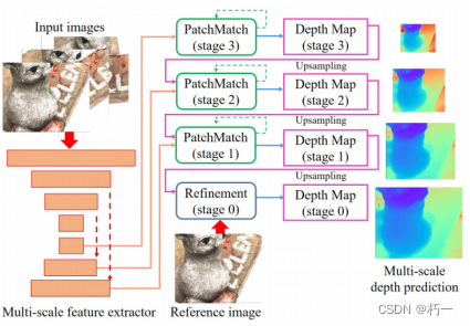
1.特征金字塔分别提取1/8、1/4、1/2特征图；
2.从低分辨率到高分辨率逐阶段细化深度图；
3.在每个阶段(stage)，使用patchmatch模块迭代推理深度图；
4.在1/1分辨率，使用一个优化网络上采样并细化深度图。

0.2 net.py

import torch
import torch.nn.functional as F


class CoreNet(torch.nn.Module):
    def __init__(self, stages, Backbone, scale, Patchmatchs, Refinenet, Calconfidence):
        super(CoreNet, self).__init__()
        self.stages = stages
        self.Backbone = Backbone
        self.scale = scale
        self.Patchmatchs = Patchmatchs
        self.Refinenet = Refinenet
        self.Confidence_regress = Calconfidence

        print('{} parameters: {}'.format(self._get_name(), sum([p.data.nelement() for p in self.parameters()])))

    def forward(self, origin_imgs, extrinsics, intrinsics, depth_range):
        """
        predict depth
        @param origin_imgs: （B,VIEW,C,H,W） view0 is ref img
        @param extrinsics: （B,VIEW,4,4）
        @param intrinsics: （B,VIEW,3,3）
        @param depth_range: (B, 2) B*(depth_min, depth_max) dtu: [425.0, 935.0] tanks: [-, -]
        @return:
        """
        origin_imgs = torch.unbind(origin_imgs.float(), 1)  # VIEW*(B,C,H,W)

        # 0. feature extraction
        featuress = [self.Backbone(img) for img in origin_imgs] #views * 3 * fea

        view_weights = None
        depths, score_volume, depth_hypos, depthss = [None,], None, None, []
        for stage in range(self.stages-1):

            # 1. get features
            features = [fea[stage] for fea in featuress]

            # 2.scale intrinsic matrix & cal proj matrix
            ref_proj, src_projs = self.scale(intrinsics, extrinsics, stage)

            # 3.patchmatch
            depths, score_volume, view_weights, depth_hypos = self.Patchmatchs[stage](
                            features, ref_proj, src_projs, depth_range, depths[-1], view_weights, score_volume, depth_hypos)

            depthss.append(depths)

        depth = self.Refinenet(origin_imgs[0], depths[-1].unsqueeze(1), depth_range)
        depthss.append(depth)

        if self.training:
            return {"depth": depthss, }

        confidence = self.Confidence_regress(score_volume)
        confidence = F.interpolate(confidence.unsqueeze(1), scale_factor=2.0, mode="nearest").squeeze(1)

        return {"depth": depths[-1], "confidence": confidence}


if __name__=="__main__":
    pass

0.3 patchmatch结构

优势：
1.3DCNN正则化要求体素中具有规则的空间结构，但多尺度方法不具备这样的结构（除第一次迭代以外）。
1）每个像素和其空间邻域的深度假设不同，难以在空间域中聚合代价（h,w维度）；
2）每个像素的深度假设不像CIDER那样均匀分布在反向深度范围内，这使得难以沿深度维度聚合成本信息（深度维度）。
2.提高效率。

0.4 patchmatch.py

from typing import List, Tuple

import torch
import torch.nn as nn
import torch.nn.functional as F

import depthhypos, propagation, evaluation


class PatchMatch(nn.Module):
    def __init__(self,
                 stage_iters: int = 2,
                 in_chs: int = 64,
                 ngroups: int = 8,
                 ndepths: int = 16,
                 propagate: bool = True,
                 propagate_neighbors: int = 16,
                 propagation_out_range: int = 2,
                 evaluate_neighbors: int = 9,
                 interval_scale: float = 0.25,
                 ) -> None:

        super(PatchMatch, self).__init__()
        self.stage_iters = stage_iters
        self.ndepths = ndepths
        self.propagate = propagate

        self.interval_scale =interval_scale

        self.Initialization =  depthhypos.DepthInitialization(ndepths)   #curve_hypos
        self.Propagation = propagation.Propagation(in_chs, propagate_neighbors, propagation_out_range)
        self.Evaluation = evaluation.Evaluation(in_chs, evaluate_neighbors, propagation_out_range, ngroups, interval_scale)

        print('{} parameters: {}'.format(self._get_name(), sum([p.data.nelement() for p in self.parameters()])))

    def forward(
            self,
            features: List[torch.Tensor],
            ref_proj: torch.Tensor,
            src_projs: List[torch.Tensor],
            depth_range: torch.Tensor,
            depth: torch.Tensor,
            view_weights: torch.Tensor,
            score: torch.Tensor,
            depth_hypos:torch.Tensor,
        ) -> Tuple[List[torch.Tensor], torch.Tensor, torch.Tensor, torch.Tensor]:

        B = depth_range.shape[0]
        depth_min, depth_max = depth_range[:, 0].float(), depth_range[:, 1].float()

        # reuse view weights
        if view_weights is not None and depth is not None:
            depth = F.interpolate(depth.unsqueeze(1).detach(), scale_factor=2, mode="nearest").squeeze(1)
            view_weights = F.interpolate(view_weights, scale_factor=2.0, mode="nearest")

        ref_feature, src_features = features[0], features[1:]  # (B,C,H,W),(nviews-1)*（B,C,H,W）
        batch, _, height, width = ref_feature.size()

        feature_weight, s, depths = None, None, []    # view_weight None , feature_weight, each iter singal cal
        for iter in range(1, self.stage_iters + 1):
            # 1.Initialization
            depth_hypos = self.Initialization(
                min_depth=depth_min,
                max_depth=depth_max,
                height=height,
                width=width,
                depth_interval_scale=self.interval_scale,
                device=depth_range.device,
                depth=depth,
            )

            # 2.Propagation
            if self.propagate:
                depth_hypos = self.Propagation(iter, ref_feature, depth_hypos,)

            # 3.Evaluation
            depth, score, view_weights\
                = self.Evaluation(iter, features, ref_proj, src_projs, view_weights, depth_hypos, depth_range)

            depths.append(depth)

        return depths, score, view_weights, depth_hypos

1. Initialization and Local Perturbation

1.首次深度假设：在深度范围[dmin，dmax]的逆深度范围进行均匀采样。有助于模型适用于大规模复杂场景。这里对深度假设加了一个随机值。
2.后续的深度假设：在深度值附近的一个给定范围假设，同样适用逆深度。围绕之前的估计值进行假设可以局部细化结果并纠正错误的估计值。

1.1 depthhypos.py

import torch
import torch.nn as nn
import torch.nn.functional as F
from typing import List, Tuple


class DepthInitialization(nn.Module):
    """Initialization Stage Class"""

    def __init__(self, patchmatch_num_sample: int = 1) -> None:
        """Initialize method

        Args:
            patchmatch_num_sample: number of samples used in patchmatch process
        """
        super(DepthInitialization, self).__init__()
        self.patchmatch_num_sample = patchmatch_num_sample

    def forward(
        self,
        min_depth: torch.Tensor,
        max_depth: torch.Tensor,
        height: int,
        width: int,
        depth_interval_scale: float,
        device: torch.device,
        depth: torch.Tensor = torch.empty(0),
    ) -> torch.Tensor:
        """Forward function for depth initialization

        Args:
            min_depth: minimum virtual depth, (B, )
            max_depth: maximum virtual depth, (B, )
            height: height of depth map
            width: width of depth map
            depth_interval_scale: depth interval scale
            device: device on which to place tensor
            depth: current depth (B, 1, H, W)

        Returns:
            depth_sample: initialized sample depth map by randomization or local perturbation (B, Ndepth, H, W)
        """
        batch_size = min_depth.size()[0]
        inverse_min_depth = 1.0 / min_depth
        inverse_max_depth = 1.0 / max_depth
        if depth is None:
            # first iteration of Patchmatch on stage 3, sample in the inverse depth range
            # divide the range into several intervals and sample in each of them
            patchmatch_num_sample = 48
            # [B,Ndepth,H,W]
            depth_sample = torch.rand(
                size=(batch_size, patchmatch_num_sample, height, width), device=device
            ) + torch.arange(start=0, end=patchmatch_num_sample, step=1, device=device).view(
                1, patchmatch_num_sample, 1, 1
            )

            depth_sample = inverse_max_depth.view(batch_size, 1, 1, 1) + depth_sample / patchmatch_num_sample * (
                inverse_min_depth.view(batch_size, 1, 1, 1) - inverse_max_depth.view(batch_size, 1, 1, 1)
            )

            return 1.0 / depth_sample

        elif self.patchmatch_num_sample == 1:
            return depth.detach()
        else:
            # otheder Patchmatch, local perturbation is performed based on previous result
            # uniform samples in an inversed depth range
            depth_sample = (
                torch.arange(-self.patchmatch_num_sample // 2, self.patchmatch_num_sample // 2, 1, device=device)
                .view(1, self.patchmatch_num_sample, 1, 1).repeat(batch_size, 1, height, width).float()
            )
            inverse_depth_interval = (inverse_min_depth - inverse_max_depth) * depth_interval_scale
            inverse_depth_interval = inverse_depth_interval.view(batch_size, 1, 1, 1)

            # print(depth.shape, inverse_depth_interval.shape)
            depth_sample = 1.0 / depth.unsqueeze(1).detach() + inverse_depth_interval * depth_sample

            depth_clamped = []
            del depth
            for k in range(batch_size):
                depth_clamped.append(
                    torch.clamp(depth_sample[k], min=inverse_max_depth[k], max=inverse_min_depth[k]).unsqueeze(0)
                )

            return 1.0 / torch.cat(depth_clamped, dim=0)

2. Adaptive Propagation

理念：将处于同一平面的邻近点的深度值添加到中心点的深度假设，有助于更快的收敛。
方法：
1.使用一个2D CNN网络，以参考图像特征图为输入，计算与中心点同一表面的邻近点其像素坐标与中心点的偏移量；
2.计算邻近点像素坐标，将其深度(上一次迭代深度图中的深度)加入当前的深度假设。

2.1 propagation.py

import torch
import torch.nn as nn
import torch.nn.functional as F

from patchbase import get_grid


class Propagation(nn.Module):
    def __init__(self,
                 in_chs,
                 neighbors,
                 dilation,
                 ):
        super(Propagation, self).__init__()

        self.neighbors = neighbors
        self.dilation = dilation
        self.grid_type = {"propagation": 1, "evaluation": 2}
        
        self.propa_conv = nn.Conv2d(
            in_channels=in_chs,
            out_channels=max(2 * neighbors, 1),
            kernel_size=3,
            stride=1,
            padding=dilation,
            dilation=dilation,
            bias=True,
        )
        nn.init.constant_(self.propa_conv.weight, 0.0)
        nn.init.constant_(self.propa_conv.bias, 0.0)

        self.propa_grid = None  #Save variables as attributes for reuse in same iter

    def forward(self,
                iter,
                ref_feature: torch.Tensor,
                depth_hypos: torch.Tensor,
                ):          #[batch, num_depth+num_neighbors, height, width]
        B, C, H, W = ref_feature.shape
        device = ref_feature.device

        if iter == 1:
            # 1. the learned additional 2D offsets for adaptive propagation
            # last iteration on stage 1 does not have propagation (photometric consistency filtering)
            propa_offset = self.propa_conv(ref_feature).view(B, 2 * self.neighbors, H * W)
            self.propa_grid = get_grid(self.grid_type["propagation"], B, H, W, propa_offset, device, self.neighbors, 0, self.dilation)

        if depth_hypos.shape[-1] == 1:

            return depth_hypos#.repeat(1, 1, H, W)

        # adaptive propagation
        # if self.propagate_neighbors > 0 and not (self.stage == 1 and iter == self.patchmatch_iteration):
        # last iteration on stage 1 does not have propagation (photometric consistency filtering)
        batch, num_depth, height, width = depth_hypos.size()
        num_neighbors = self.propa_grid.size()[1] // height

        # num_depth//2 is nearest depth map
        propagate_depth_hypos = F.grid_sample(
            depth_hypos[:, num_depth // 2, :, :].unsqueeze(1), self.propa_grid,
            mode="bilinear", padding_mode="border", align_corners=False
        ).view(batch, num_neighbors, height, width)

        return torch.sort(torch.cat((depth_hypos, propagate_depth_hypos), dim=1), dim=1)[0]

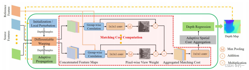
3.Adaptive Evaluation

3.1代价体的构建

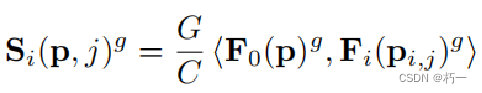
1.使用可微的单应性变化扭曲特征图；
2.使用分组内积的方式聚合代价体，并引入可见性权重（使用一个共享权重的2D CNN网络计算，只使用第一次计算的可见性权重，之后直接使用或上采样使用）；
3.计算加权平均值。

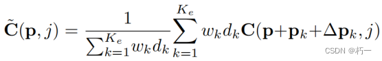
3.2 Adaptive Spatial Cost Aggregation

理念：与自适应传播相似，使用邻域点计算匹配代价。（传统的MVS匹配算法通常会在一个空间窗口上聚合代价，以提高匹配鲁棒性和隐式平滑效果等。）
方法：
1.使用一个2D CNN网络计算同一平面邻域点的坐标偏移量。
2.计算邻域点坐标并计算其权重；
2.使用一个相似性计算网络（3D CNN，简化了正则化网络，将特征维度降为1）计算概率体；
3.根据邻域点计算加权概率体。

3.3 Depth Regression

1.深度图：使用常用的soft argmin
2.概率图：也是用常用的四邻域加和。

3.4 evaluation.py

from typing import List, Tuple
import torch
import torch.nn as nn
import torch.nn.functional as F

from patchbase import get_grid, ConvBnReLU3D


class Evaluation(nn.Module):
    def __init__(self,
                 in_chs,
                 neighbors,  #9
                 dilation,
                 ngroups: int,
                 interval_scale,
                 ):
        super(Evaluation, self).__init__()

        self.ngroups = ngroups
        self.neighbors = neighbors
        self.dilation = dilation
        self.grid_type = {"propagation": 1, "evaluation": 2}

        self.interval_scale = interval_scale

        # adaptive spatial cost aggregation (adaptive evaluation)
        self.Eval_conv = nn.Conv2d(
            in_channels=in_chs,
            out_channels=2 * neighbors,
            kernel_size=3,
            stride=1,
            padding=dilation,
            dilation=dilation,
            bias=True,
        )
        nn.init.constant_(self.Eval_conv.weight, 0.0)
        nn.init.constant_(self.Eval_conv.bias, 0.0)

        self.Feature_weight_conv = nn.Sequential(
            ConvBnReLU3D(in_channels=ngroups, out_channels=16, kernel_size=1, stride=1, pad=0),
            ConvBnReLU3D(in_channels=16, out_channels=8, kernel_size=1, stride=1, pad=0),
            nn.Conv3d(in_channels=8, out_channels=1, kernel_size=1, stride=1, padding=0)
        )

        self.Pixel_wise_conv = nn.Sequential(
            ConvBnReLU3D(in_channels=ngroups, out_channels=16, kernel_size=1, stride=1, pad=0),
            ConvBnReLU3D(in_channels=16, out_channels=8, kernel_size=1, stride=1, pad=0),
            nn.Conv3d(in_channels=8, out_channels=1, kernel_size=1, stride=1, padding=0),
        )

        self.Similaritynet = nn.Sequential(
            ConvBnReLU3D(in_channels=ngroups, out_channels=16, kernel_size=1, stride=1, pad=0),
            ConvBnReLU3D(in_channels=16, out_channels=8, kernel_size=1, stride=1, pad=0),
            nn.Conv3d(in_channels=8, out_channels=1, kernel_size=1, stride=1, padding=0),
        )

        self.sigmoid = nn.Sigmoid()
        self.softmax = nn.Softmax(dim=1)

        self.eval_grid = None   # Save variables as attributes for reuse in same iter
        self.feature_weight = None

    def forward(self,
                iter,
                features: List[torch.Tensor],
                ref_proj,
                src_projs,
                view_weights,
                depth_hypos: torch.Tensor,
                depth_range,
                ):
        ref_feature, src_features = features[0], features[1:]  # (B,C,H,W),(nviews-1)*（B,C,H,W）
        B, C, H, W = ref_feature.shape
        ndepths = depth_hypos.shape[1]
        device = ref_feature.device
        depth_min, depth_max = depth_range[:, 0].float(), depth_range[:, 1].float()

        if iter == 1:
            # 1. the learned additional 2D offsets for adaptive spatial cost aggregation (adaptive evaluation)
            eval_offset = self.Eval_conv(ref_feature)
            eval_offset = eval_offset.view(B, 2*self.neighbors, H * W)    #2 * evaluate_neighbors
            self.eval_grid = get_grid(self.grid_type["evaluation"], B, H, W, eval_offset, device, 0, self.neighbors, self.dilation)

            # 2. feature_weight [B, evaluate_neighbors, H, W]
            weight = F.grid_sample(ref_feature.detach(), self.eval_grid,
                                   mode="bilinear", padding_mode="border", align_corners=False)
            weight = weight.view(B, self.ngroups, C // self.ngroups, self.neighbors, H, W)
            ref_feature = ref_feature.view(B, self.ngroups, C // self.ngroups, H, W).unsqueeze(3)
            weight = (weight * ref_feature).mean(2) # [B,G,Neighbor,H,W]
            self.feature_weight = self.sigmoid(self.Feature_weight_conv(weight.detach()).squeeze(1))     #[B,Neighbor,H,W]

        # # 3. weights for adaptive spatial cost aggregation in adaptive evaluation
        inverse_depth_min = 1.0 / depth_min
        inverse_depth_max = 1.0 / depth_max

        # normalization
        x = 1.0 / depth_hypos
        x = (x - inverse_depth_max.view(B, 1, 1, 1)) / (inverse_depth_min - inverse_depth_max).view(B, 1, 1, 1)

        x1 = F.grid_sample(
            x.detach(), self.eval_grid.detach(), mode="bilinear", padding_mode="border", align_corners=False
        ).view(B, ndepths, self.neighbors, H, W)

        # [B,Ndepth,N_neighbors,H,W]
        x1 = torch.abs(x1 - x.unsqueeze(2)) / self.interval_scale
        del x

        # sigmoid output approximate to 1 when x=4
        depth_weight =  torch.sigmoid(4.0 - 2.0 * x1.clamp(min=0, max=4)).detach()
        del x1
        weight = depth_weight * self.feature_weight.unsqueeze(1)
        weight = weight / torch.sum(weight, dim=2).unsqueeze(2)  # [B,Ndepth,1,H,W]
        del depth_weight

        # 4. warp & aggrate
        # evaluation, outputs regressed depth map and pixel-wise view weights which will
        # be used for subsequent iterations
        ref_volume = ref_feature.view(B, self.ngroups, C // self.ngroups, 1, H, W)

        view_weight_sum, view_weights_cur, similarity_sum = 1e-5, [], 0.0
        for n, (src_feature, src_proj) in enumerate(zip(src_features, src_projs)):
            warped_volume = differentiable_warping(src_feature, src_proj, ref_proj, depth_hypos)
            warped_volume = warped_volume.view(B, self.ngroups, C // self.ngroups, ndepths, H, W)
            similarity = (warped_volume * ref_volume).mean(2)
            del warped_volume

            if view_weights is None:
                view_weight = self.Pixel_wise_conv(similarity)
                view_weight = torch.max(self.sigmoid(view_weight.squeeze(1)), dim=1)[0].unsqueeze(1)
                view_weights_cur.append(view_weight)
            else:
                # reuse the pixel-wise view weight from first iteration of Patchmatch on stage 3
                view_weight = view_weights[:, n].unsqueeze(1)  # [B,1,H,W]

            similarity_sum += similarity * view_weight.unsqueeze(1)
            view_weight_sum += view_weight.unsqueeze(1)
            del similarity, view_weight

        similarity = similarity_sum.div_(view_weight_sum)  # [B, G, Ndepth, H, W]
        del similarity_sum, view_weight_sum

        if view_weights is None:
            view_weights = torch.cat(view_weights_cur, dim=1)  # [B,4,H,W], 4 is the number of source views

        # 5. adaptive spatial cost aggregation, apply softmax to get probability
        score = self.Similaritynet(similarity).squeeze(1)  # [B, Ndepth, H, W]
        score = F.grid_sample(score, self.eval_grid, mode="bilinear", padding_mode="border", align_corners=False) \
            .view(B, ndepths, self.neighbors, H, W)
        score = torch.sum(score * weight, dim=2) ## [B,D,H,W]
        score = self.softmax(score)

        # 6. depth regression: expectation
        depth = torch.sum(depth_hypos * score, dim=1)

        return depth, score, view_weights.detach()


def differentiable_warping(
    src_fea: torch.Tensor, src_proj: torch.Tensor, ref_proj: torch.Tensor, depth_samples: torch.Tensor
):
    """Differentiable homography-based warping, implemented in Pytorch.

    Args:
        src_fea: [B, C, H, W] source features, for each source view in batch
        src_proj: [B, 4, 4] source camera projection matrix, for each source view in batch
        ref_proj: [B, 4, 4] reference camera projection matrix, for each ref view in batch
        depth_samples: [B, Ndepth, H, W] virtual depth layers
    Returns:
        warped_src_fea: [B, C, Ndepth, H, W] features on depths after perspective transformation
    """

    batch, channels, height, width = src_fea.shape
    num_depth = depth_samples.shape[1]

    with torch.no_grad():
        proj = torch.matmul(src_proj, torch.inverse(ref_proj))
        rot = proj[:, :3, :3]  # [B,3,3]
        trans = proj[:, :3, 3:4]  # [B,3,1]

        y, x = torch.meshgrid(
            [
                torch.arange(0, height, dtype=torch.float32, device=src_fea.device),
                torch.arange(0, width, dtype=torch.float32, device=src_fea.device),
            ]
        )
        y, x = y.contiguous(), x.contiguous()
        y, x = y.view(height * width), x.view(height * width)
        xyz = torch.stack((x, y, torch.ones_like(x)))  # [3, H*W]
        xyz = torch.unsqueeze(xyz, 0).repeat(batch, 1, 1)  # [B, 3, H*W]
        rot_xyz = torch.matmul(rot, xyz)  # [B, 3, H*W]

        rot_depth_xyz = rot_xyz.unsqueeze(2).repeat(1, 1, num_depth, 1) * depth_samples.view(
            batch, 1, num_depth, height * width
        )  # [B, 3, Ndepth, H*W]
        proj_xyz = rot_depth_xyz + trans.view(batch, 3, 1, 1)  # [B, 3, Ndepth, H*W]
        # avoid negative depth
        negative_depth_mask = proj_xyz[:, 2:] <= 1e-3
        proj_xyz[:, 0:1][negative_depth_mask] = float(width)
        proj_xyz[:, 1:2][negative_depth_mask] = float(height)
        proj_xyz[:, 2:3][negative_depth_mask] = 1.0
        proj_xy = proj_xyz[:, :2, :, :] / proj_xyz[:, 2:3, :, :]  # [B, 2, Ndepth, H*W]
        proj_x_normalized = proj_xy[:, 0, :, :] / ((width - 1) / 2) - 1  # [B, Ndepth, H*W]
        proj_y_normalized = proj_xy[:, 1, :, :] / ((height - 1) / 2) - 1
        proj_xy = torch.stack((proj_x_normalized, proj_y_normalized), dim=3)  # [B, Ndepth, H*W, 2]
        grid = proj_xy

    warped_src_fea = F.grid_sample(
        src_fea,
        grid.view(batch, num_depth * height, width, 2),
        mode="bilinear",
        padding_mode="zeros",
        align_corners=True,
    )

    return warped_src_fea.view(batch, channels, num_depth, height, width)

4. Refine

精度已经足够，没必要在1/1分辨率使用patchmatch。设计了一个深度残差网络。为了避免对某个深度比例产生偏差，将输入深度贴图预缩放到[0,1]范围内，并在细化后将其转换回。细化网络输出一个残差，该残差与上采样的深度相加，以获得细化的深度图。

4.1 refine.py

import torch
import torch.nn as nn
import torch.nn.functional as F

from patchbase import ConvBNReLU


class RefineNet(nn.Module):
    def __init__(self):
        super(RefineNet, self).__init__()
        self.conv_img = ConvBNReLU(3, 8)
        self.conv_depth = nn.Sequential(
            ConvBNReLU(1, 8),
            ConvBNReLU(8, 8),
            nn.ConvTranspose2d(8, 8, 3, 2, 1, 1, bias=False),
            nn.BatchNorm2d(8),
            nn.ReLU(inplace=True),
        )

        self.conv_res = nn.Sequential(
            ConvBNReLU(16, 8),
            nn.Conv2d(8, 1, 3, 1, 1, bias=False),
        )

        print('{} parameters: {}'.format(self._get_name(), sum([p.data.nelement() for p in self.parameters()])))

    def forward(self,
                ref_img: torch.Tensor,
                depth: torch.Tensor,
                depth_range: torch.Tensor,
                ) -> torch.Tensor:
        """

        @param ref_img: (B, 3, H, W)
        @param depth: (B, 1, H/2, W/2)
        @param depth_range: (B, 2)   B*(depth_min, depth_max)
        @return:depth map (B, H, W)
        """
        B, _, H, W = ref_img.shape
        depth = depth.unsqueeze(1).detach()
        depth_min, depth_max = depth_range[:, 0].float(), depth_range[:, 1].float()
        # pre-scale the depth map into [0,1]
        depth = (depth - depth_min.view(B, 1, 1, 1)) / ((depth_max - depth_min).view(B, 1, 1, 1)) #* 10

        ref_img = self.conv_img(ref_img)
        depth_conv = self.conv_depth(depth)

        res = self.conv_res(torch.cat([ref_img,depth_conv], dim=1))
        depth = F.interpolate(depth, scale_factor=2, mode="bilinear", align_corners=True) + res
        # convert the normalized depth back
        depth =  depth_min.view(B, 1, 1, 1)+\
                 depth * (depth_max.view(B, 1, 1, 1) - depth_min.view(B, 1, 1, 1))

        return depth.squeeze(1)

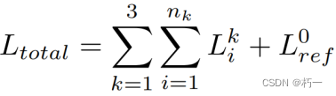
5. Loss

所有阶段，所有迭代的深度图都计算损失。

三、Experiment

1. Robust Training Strategy

通常MVS网络使用最佳的视图进行训练。然而，选定的源视图与参考视图具有很强的可见性相关性，这可能会影响像素级视图权重网络的训练。因此，从十个最佳视图中随机选择四个进行训练。该策略增加了训练时的多样性，动态地扩充了数据集，提高了泛化性能。此外，对那些具有弱可见性相关性的随机源视图进行训练，可以进一步增强可见性估计的稳健性。

2. Train args

1.图像分辨率：640x512
2.视角数：5
3.迭代次数：2、2、1
4.初始的深度平面数：48
5.之后的深度平面数：16、8、8
6.传播：在前两个stage传播
7.epoch = 8
8.lr = 0.001
9.batch size = 4
10.device:2个Nvidia GTX 1080Ti GPU

四、Other code

1.patchbase.py

from typing import List, Tuple

import torch
import torch.nn as nn
import torch.nn.functional as F


class ConvBnReLU3D(nn.Module):
    def __init__(
        self,
        in_channels: int,
        out_channels: int,
        kernel_size: int = 3,
        stride: int = 1,
        pad: int = 1,
        dilation: int = 1,
    ) -> None:

        super(ConvBnReLU3D, self).__init__()
        self.conv = nn.Conv3d(
            in_channels, out_channels, kernel_size, stride=stride, padding=pad, dilation=dilation, bias=False
        )
        self.bn = nn.BatchNorm3d(out_channels)

    def forward(self, x: torch.Tensor) -> torch.Tensor:

        return F.relu(self.bn(self.conv(x)), inplace=True)


def get_grid(
        grid_type: int,
        batch: int,
        height: int,
        width: int,
        offset: torch.Tensor,
        device: torch.device,
        propagate_neighbors: int,
        evaluate_neighbors: int,
        dilation: int,
) -> torch.Tensor:
    """Compute the offset for adaptive propagation or spatial cost aggregation in adaptive evaluation

    Args:
        grid_type: type of grid - propagation (1) or evaluation (2)
        batch: batch size
        height: grid height
        width: grid width
        offset: grid offset
        device: device on which to place tensor

    Returns:
        generated grid: in the shape of [batch, propagate_neighbors*H, W, 2]
    """
    grid_types = {"propagation": 1, "evaluation": 2}

    if grid_type == grid_types["propagation"]:
        if propagate_neighbors == 4:  # if 4 neighbors to be sampled in propagation
            original_offset = [[-dilation, 0], [0, -dilation], [0, dilation], [dilation, 0]]
        elif propagate_neighbors == 8:  # if 8 neighbors to be sampled in propagation
            original_offset = [
                [-dilation, -dilation],
                [-dilation, 0],
                [-dilation, dilation],
                [0, -dilation],
                [0, dilation],
                [dilation, -dilation],
                [dilation, 0],
                [dilation, dilation],
            ]
        elif propagate_neighbors == 16:  # if 16 neighbors to be sampled in propagation
            original_offset = [
                [-dilation, -dilation],
                [-dilation, 0],
                [-dilation, dilation],
                [0, -dilation],
                [0, dilation],
                [dilation, -dilation],
                [dilation, 0],
                [dilation, dilation],
            ]
            for i in range(len(original_offset)):
                offset_x, offset_y = original_offset[i]
                original_offset.append([2 * offset_x, 2 * offset_y])
        else:
            raise NotImplementedError
    elif grid_type == grid_types["evaluation"]:
        dilation = dilation - 1  # dilation of evaluation is a little smaller than propagation
        if evaluate_neighbors == 9:  # if 9 neighbors to be sampled in evaluation
            original_offset = [
                [-dilation, -dilation],
                [-dilation, 0],
                [-dilation, dilation],
                [0, -dilation],
                [0, 0],
                [0, dilation],
                [dilation, -dilation],
                [dilation, 0],
                [dilation, dilation],
            ]
        elif evaluate_neighbors == 17:  # if 17 neighbors to be sampled in evaluation
            original_offset = [
                [-dilation, -dilation],
                [-dilation, 0],
                [-dilation, dilation],
                [0, -dilation],
                [0, 0],
                [0, dilation],
                [dilation, -dilation],
                [dilation, 0],
                [dilation, dilation],
            ]
            for i in range(len(original_offset)):
                offset_x, offset_y = original_offset[i]
                if offset_x != 0 or offset_y != 0:
                    original_offset.append([2 * offset_x, 2 * offset_y])
        else:
            raise NotImplementedError
    else:
        raise NotImplementedError

    with torch.no_grad():
        y_grid, x_grid = torch.meshgrid(
            [
                torch.arange(0, height, dtype=torch.float32, device=device),
                torch.arange(0, width, dtype=torch.float32, device=device),
            ]
        )
        y_grid, x_grid = y_grid.contiguous().view(height * width), x_grid.contiguous().view(height * width)
        xy = torch.stack((x_grid, y_grid))  # [2, H*W]
        xy = torch.unsqueeze(xy, 0).repeat(batch, 1, 1)  # [B, 2, H*W]

    xy_list = []
    for i in range(len(original_offset)):
        original_offset_y, original_offset_x = original_offset[i]
        offset_x = original_offset_x + offset[:, 2 * i, :].unsqueeze(1)
        offset_y = original_offset_y + offset[:, 2 * i + 1, :].unsqueeze(1)
        xy_list.append((xy + torch.cat((offset_x, offset_y), dim=1)).unsqueeze(2))

    xy = torch.cat(xy_list, dim=2)  # [B, 2, 9, H*W]

    del xy_list
    del x_grid
    del y_grid

    x_normalized = xy[:, 0, :, :] / ((width - 1) / 2) - 1
    y_normalized = xy[:, 1, :, :] / ((height - 1) / 2) - 1
    del xy
    grid = torch.stack((x_normalized, y_normalized), dim=3)  # [B, 9, H*W, 2]
    del x_normalized
    del y_normalized
    return grid.view(batch, len(original_offset) * height, width, 2)


class ConvBNReLU(nn.Module):
    def __init__(self,
                 inchs: int,
                 outchs: int,
                 kernel_size: int = 3,
                 stride: int = 1,
                 padding: int = 1,
                 groups: int = 1,
                 bias: bool = False,
                 ) -> None:
        super(ConvBNReLU, self).__init__()
        self.conv = nn.Conv2d(inchs, outchs, kernel_size, stride, (kernel_size-1)//2, groups=groups, bias=bias)
        self.bn = nn.BatchNorm2d(outchs)
        self.relu = nn.ReLU(inplace=True)

    def forward(self,
                x: torch.Tensor,
                ) -> torch.Tensor:
        return self.relu(self.bn(self.conv(x)))

2. config.py(设置参数，创建网络)

""" 
net args
"""
import torch.nn as nn
import net, patchmatch
import scale, backbone, regress, refine
stages = 4
# scale matrix method
scale = scale.scale_cam
# Feature map extraction network
out_chs = [8, 16, 32, 64]
Backbone= backbone.FPN_4Scales(out_chs)
# patchmatch init
stage_iters = [2, 2, 1]
in_chs = list(reversed(out_chs[1:]))
vec_dim = 2
ngroups = [8, 8, 4]   
ndepths = [16, 8, 8]
propagate = [True, True, False]
propagation_out_range = [2, 4, 6]
propagate_neighbors = [16, 8, 0]
evaluate_neighbors = [9, 9, 9]

interval_scale = [0.025, 0.0125, 0.005]

Patchmatchs = nn.ModuleList([
    patchmatch.PatchMatch(
        stage_iters[s],
        in_chs[s],
        ngroups[s],
        ndepths[s],
        propagate[s],
        propagate_neighbors[s],
        propagation_out_range[s],
        evaluate_neighbors[s],
        interval_scale[s],
    )
    for s in range(stages-1)
])

# refine net
Refinenet = refine.Refinement()
# confidence regress
Calconfidence = regress.confidence_regress

# # model
model = net.CoreNet(stages, Backbone, scale, Patchmatchs, Refinenet, Calconfidence)

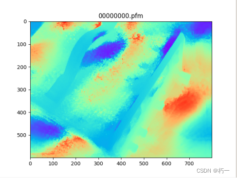
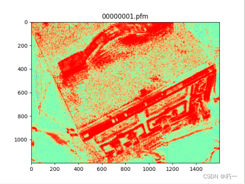
五、Test

训练一个epoch的结果：

深度图：

概率图：

参考文献：
[1] Wang F, Galliani S, Vogel C, et al. Patchmatchnet: Learned multi-view patchmatch stereo[C]//Proceedings of the IEEE/CVF Conference on Computer Vision and Pattern Recognition. 2021: 14194-14203.