利用pytorch搭建神经网络

拟合散点图

• 简单介绍
  首先我们需要构造一些“假”的数据（即一些零散的点），主要的任务就是在这些假的数据点中拟合出一条曲线，使这条曲线尽可能地“穿过”所有的点。
• 制作数据集
  我们在y=sin(x)+b这条曲线附近取一些点，使b具有随机性，因为在生活中大部分数据不可能精确到直接可以满足一条公式，基本所有的都是尽可能地去拟合数据。
  

import torch
import matplotlib.pyplot as plt

#制作假的数据集
x = torch.unsqueeze(torch.linspace(-1,1,100), dim=1)
y = torch.asin(x) + 0.2*torch.rand(x.size())

plt.scatter(x.data.numpy(), y.data.numpy())
plt.show()

• 搭建神经网络
  这里的大概流程直接可以在pytorch的官方文档中找到，这是一份中文文档
  
  具体搭建网络时需要继承torch中的Model类，类中主要有两个函数,init函数的作用是设置神经网络的每一层，即告诉我们每一层是干嘛的，都长啥样。而forward函数则相当于实战，传入数据，输出结果。

import torch
import torch.nn.functional as F

class Net(torch.nn.Module):
    def __init__(self, n_features, hiddens, o_features):
        #这一行代码可以不用管它到底是干什么的，只要知道如果要搭建网络必须这么干就完事
        #如果非要搞懂，可以看一下下方的链接
        #https://blog.csdn.net/wltsysterm/article/details/104440387
        super(Net, self).__init__()
        self.hidden = torch.nn.Linear(n_features, hiddens)
        self.predict = torch.nn.Linear(hiddens, o_features)

    def forward(self, x):
        x = self.hidden(x)
        x = F.relu(x)
        x = self.predict(x)

        return x

#构建一个网络
net = Net(n_features=1, hiddens=128, o_features=1)
print(net)
'''
Net(
  (hidden): Linear(in_features=1, out_features=128, bias=True)
  (predict): Linear(in_features=128, out_features=1, bias=True)
)
'''

• 训练网络
  网络搭建好了，在训练网络之前，为了达到良好的效果，还需要选择适当的优化器，并且设置一些超参数，再选择合适的损失函数来表示误差，鉴定模型的优劣。最后通过循环不断将提前准备好的假数据喂给网络。

#设置优化器
optimizer = torch.optim.SGD(net.parameters(), lr=0.1)
#误差计算
loss_func = torch.nn.MSELoss()

#训练
for t in range(100):
    #预测值
    prediction = net(x)
    loss = loss_func(prediction, y)
    #清空梯度参数
    optimizer.zero_grad()
    #误差反向传播更新参数
    loss.backward()
    #更新网络参数
    optimizer.step()

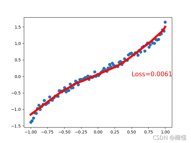
• 可视化拟合结果
  为了能够直观的看出最后的拟合效果，将预测到的结果与原来的散点图绘制在一张图上。在这里经过多次训练选取了效果较好的一次展示。
  

#可视化最后拟合出来的曲线
plt.figure()
plt.scatter(x.data.numpy(), y.data.numpy(), color='blue')
plt.plot(x.data.numpy(), prediction.data.numpy(), 'r-', lw=5)
plt.text(0.5, 0, 'Loss=%.4f' % loss.data.numpy(), fontdict={'size': 15, 'color':  'red'})
plt.scatter(x.data.numpy(), y.data.numpy())
plt.show()

最后附上全部代码

import torch
import matplotlib.pyplot as plt
import torch.nn.functional as F

#制作假的数据集
x = torch.unsqueeze(torch.linspace(-1,1,100), dim=1)
y = torch.asin(x) + 0.2*torch.rand(x.size())


class Net(torch.nn.Module):
    def __init__(self, n_features, hiddens, o_features):
        #这一行代码可以不用管它到底是干什么的，只要知道如果要搭建网络必须这么干就完事
        #如果非要搞懂，可以看一下本节下方的链接
        super(Net, self).__init__()
        self.hidden = torch.nn.Linear(n_features, hiddens)
        self.predict = torch.nn.Linear(hiddens, o_features)

    def forward(self, x):
        x = self.hidden(x)
        x = F.relu(x)
        x = self.predict(x)

        return x

#构建一个网络
net = Net(n_features=1, hiddens=128, o_features=1)
print(net)
'''
Net(
  (hidden): Linear(in_features=1, out_features=128, bias=True)
  (predict): Linear(in_features=128, out_features=1, bias=True)
)
'''

#设置优化器
optimizer = torch.optim.SGD(net.parameters(), lr=0.1)
#误差计算
loss_func = torch.nn.MSELoss()

#训练
for t in range(100):
    #预测值
    prediction = net(x)
    loss = loss_func(prediction, y)
    #清空梯度参数
    optimizer.zero_grad()
    #误差反向传播更新参数
    loss.backward()
    #更新网络参数
    optimizer.step()

#可视化最后拟合出来的曲线
plt.figure()
plt.scatter(x.data.numpy(), y.data.numpy(), color='blue')
plt.plot(x.data.numpy(), prediction.data.numpy(), 'r-', lw=5)
plt.text(0.5, 0, 'Loss=%.4f' % loss.data.numpy(), fontdict={'size': 15, 'color':  'red'})
plt.scatter(x.data.numpy(), y.data.numpy())
plt.show()