线性回归——多元线性回归

理论推导

预测值：${\theta }_0$+${\theta }_1$$x_1$+…+${\theta }_n$$x_n$
       \qquad\;\;\; =${\theta }_0$$x_0$+${\theta }_1$$x_1$+…+${\theta }_n$*$x_n$ \qquad\qquad\qquad ($x_0$=1)
       \qquad\;\;\; =${\theta }^T$x
一个样本的误差：（$y^{(i)}$ - ${\theta }^T$$x^{(i)}$）
整个样本集代价函数（最小二乘法）：J(θ)=$\frac{1}{2m}$${\sum }_{i=1}^m$$（y^{(i)}-{\theta }^T\ast x^{(i)}{）}^2$
采用梯度下降法进行优化：
${\theta }_0$=${\theta }_0$-$\frac{1}{m}$${\sum }_{i=1}^m$$（y^{(i)}-{\theta }^T\ast x^{(i)}）$×（-$x_0$）
${\theta }_1$=${\theta }_1$-$\frac{1}{m}$${\sum }_{i=1}^m$$（y^{(i)}-{\theta }^T\ast x^{(i)}）$×（-$x_1$）
.
${\theta }_n$=${\theta }_n$-$\frac{1}{m}$${\sum }_{i=1}^m$$（y^{(i)}-{\theta }^T\ast x^{(i)}）$×（-$x_n$）

代码

梯度下降法-二元线性回归-3D绘图

import numpy as np
import matplotlib.pyplot as plt
from mpl_toolkits.mplot3d import Axes3D

#读入数据
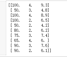
data=np.genfromtxt("Delivery.csv",delimiter=',')
print(data)

#切分数据
#样本个特征值-不要最后一列
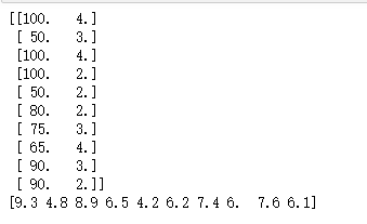
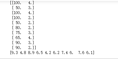
x=data[:,:-1]
#真实值-最后一列
y=data[:,-1]
print(x)
print(y)

#学习率
learning_rate=0.0001
#待确定参数
th0=0
th1=0
th2=0
#迭代次数
loop=1000

#梯度下降法——二元:y=th0+th1*x[0]*th2*x[1]
def gradient_descent(x,y,th0,th1,th2,learning_rate,loop):
    #数据总量
    m=float(len(x))
    for i in range(loop):
        #临时变量
        th0_temp=0
        th1_temp=0
        th2_temp=0
        for j in range(0,len(x)):
            th0_temp+=-(1/m)*(y[j]-th0-th1*x[j,0]-th2*x[j,1])
            #求导有负号
            th1_temp+=-(1/m)*(y[j]-th0-th1*x[j,0]-th2*x[j,1])*x[j,0]
            th2_temp+=-(1/m)*(y[j]-th0-th1*x[j,0]-th2*x[j,1])*x[j,1]
        #更新三个参数
        th0-=learning_rate*th0_temp
        th1-=learning_rate*th1_temp
        th2-=learning_rate*th2_temp
    return th0,th1,th2

#损失
def error (th0,th1,th2,x,y):
    totalError=0
    for i in range(len(x)):
        totalError+=(y[i]-th0-th1*x[i,0]-th2*x[i,1])**2
    return totalError/float(len(x))

th0,th1,th2=gradient_descent(x,y,th0,th1,th2,learning_rate,loop)
print("{0},{1},{2},{3}".format(th0,th1,th2,error(th0,th1,th2,x,y)))

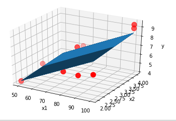
#画图-3d
ax=plt.figure().add_subplot(111,projection='3d')
#散点图
ax.scatter(x[:,0],x[:,1],y,c='r',marker='o',s=100)
x1=x[:,0]
x2=x[:,1]
#生成网格矩阵
x1,x2=np.meshgrid(x1,x2)
z=th0+th1*x1+th2*x2
ax.plot_surface(x1,x2,z)
#设置坐标轴
ax.set_xlabel('x1')
ax.set_ylabel('x2')
ax.set_zlabel('y')
#图像显示
plt.show()

sklearn-多元线性回归

import numpy as np
from sklearn import linear_model
import matplotlib.pyplot as plt
from mpl_toolkits.mplot3d import Axes3D

#读入数据
data=np.genfromtxt("Delivery.csv",delimiter=',')
print(data)

#切分数据
x=data[:,:-1]
y=data[:,-1]
print(x)
print(y)

#创建模型
model=linear_model.LinearRegression()
#填入参数
model.fit(x,y)

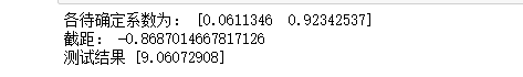
#输出待确定的系数
print("各待确定系数为：",model.coef_)
#输出截距=偏置
print("截距：",model.intercept_)
#测试
test=[[102,4]]
answer_test=model.predict(test)
print("测试结果",answer_test)

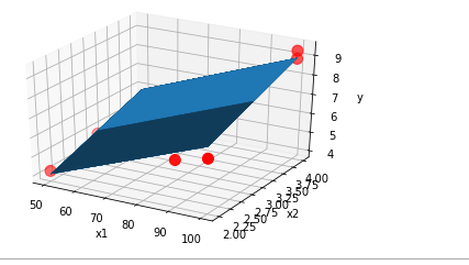
#画图-3d
ax=plt.figure().add_subplot(111,projection='3d')
#散点图
ax.scatter(x[:,0],x[:,1],y,c='r',marker='o',s=100)
x1=x[:,0]
x2=x[:,1]
#生成网格矩阵
x1,x2=np.meshgrid(x1,x2)
z=model.intercept_+x1*model.coef_[0]+x2*model.coef_[1]
#画3d图
ax.plot_surface(x1,x2,z)
#设置坐标轴
ax.set_xlabel('x1')
ax.set_ylabel('x2')
ax.set_zlabel('y')
#图像显示
plt.show()