


泊松分布:
模型:假设单位时间内发生时间
λ
\lambda
λ次,求单位时间内事件发生x次的概率。
分布函数:
p
(
x
)
=
e
−
λ
λ
x
x
!
p(x)=\frac{e^{-\lambda}\lambda^x}{x!}
p(x)=x!e−λλx
矩母函数:
M
x
(
t
)
=
E
(
e
t
x
)
=
∑
x
=
0
∞
e
t
x
e
−
λ
λ
x
x
!
M_x(t)=E(e^{tx})=\sum_{x=0}^∞ \frac{e^{tx}e^{-\lambda}\lambda^x}{x!}
Mx(t)=E(etx)=x=0∑∞x!etxe−λλx
期
望
E
(
x
)
=
λ
;
方
差
V
a
r
(
x
)
=
λ
期望E(x)=\lambda \ ;\ 方差Var(x)=\lambda
期望E(x)=λ ; 方差Var(x)=λ
似然函数:
L
=
−
n
λ
+
∑
i
=
1
n
(
x
i
l
n
λ
−
l
n
x
i
)
L=-n\lambda+\sum_{i=1}^n(x_iln\lambda-lnx_i)
L=−nλ+i=1∑n(xilnλ−lnxi)
性质:
x
1
∼
P
o
i
s
s
o
n
(
λ
1
)
,
x
2
∼
P
o
i
s
s
o
n
(
λ
2
)
x_1\sim Poisson(\lambda_1) \ ,x_2\sim Poisson(\lambda_2)
x1∼Poisson(λ1) ,x2∼Poisson(λ2)
x
1
+
x
2
∼
P
o
i
s
s
o
n
(
λ
1
+
λ
2
)
x_1+x_2\sim Poisson(\lambda_1+\lambda_2)
x1+x2∼Poisson(λ1+λ2)
用matplotlib验证这一性质:
import numpy as np
import matplotlib.pyplot as plt

plt.xlim(0,30)
plt.ylim(0.00,0.20)
sample1 = np.random.poisson(lam=5, size=10000)
sample2 = np.random.poisson(lam=10, size=10000)
sample3 = np.random.poisson(lam=15, size=10000)
pillar=30
s1=plt.hist(sample1,rwidth=0.9,alpha=0.6,density=True,label="x1",bins=pillar,range=[0,pillar])
plt.plot(s1[1][0:pillar],s1[0],'blue')
s2=plt.hist(sample2,rwidth=0.9,alpha=0.6,density=True,label="x2",bins=pillar,range=[0,pillar])
plt.plot(s2[1][0:pillar],s2[0],'orange')
s3=plt.hist(sample3,rwidth=0.9,alpha=0.6,density=True,label="x3",bins=pillar,range=[0,pillar])
plt.plot(s3[1][0:pillar],s3[0],'g')
s4=plt.hist(sample1+sample2,rwidth=0.9,alpha=0.6,density=True,label="x3=x1+x2",bins=pillar,range=[0,pillar])
plt.plot(s4[1][0:pillar],s4[0],'r')
plt.legend()
plt.show()

泊松分布与二项分布的关系:
二项分布:
C
n
x
p
x
(
1
−
p
)
n
−
x
C_n^x p^x(1-p)^{n-x}
Cnxpx(1−p)n−x
二者关系:
lim
n
→
∞
(
x
n
)
p
x
(
1
−
p
)
n
−
x
=
e
−
λ
λ
x
x
!
\lim_{n\to∞}\big(_x^n\big)p^x(1-p)^{n-x}=\frac{e^{-\lambda }\lambda^x}{x!}
n→∞lim(xn)px(1−p)n−x=x!e−λλx
证明:
令
p
=
λ
n
令p=\frac{\lambda}{n}
令p=nλ
lim
n
→
∞
(
x
n
)
(
λ
n
)
x
(
1
−
λ
n
)
n
−
x
\lim_{n\to∞}\big(_x^n\big)(\frac{\lambda}{n})^x(1-\frac{\lambda}{n})^{n-x}
n→∞lim(xn)(nλ)x(1−nλ)n−x
=
lim
n
→
∞
n
!
x
!
(
n
−
x
)
!
(
λ
n
)
x
(
1
−
λ
n
)
n
−
x
=\lim_{n\to∞}\frac{n!}{x!(n-x)!}(\frac{\lambda}{n})^x(1-\frac{\lambda}{n})^{n-x}
=n→∞limx!(n−x)!n!(nλ)x(1−nλ)n−x
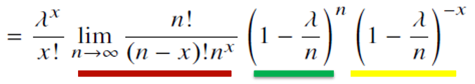
=
λ
x
x
!
lim
n
→
∞
n
!
x
!
(
n
−
x
)
!
(
1
−
λ
n
)
n
(
1
−
λ
n
)
n
−
x
=\frac{\lambda^x}{x!} \lim_{n\to∞}\frac{n!}{x!(n-x)!}(1-\frac{\lambda}{n})^n(1-\frac{\lambda}{n})^{n-x}
=x!λxn→∞limx!(n−x)!n!(1−nλ)n(1−nλ)n−x

import numpy as np
import matplotlib.pyplot as plt


def draw(n,p,lam):
    plt.title("n={}, p={}, $\lambda$={}".format(n,p,lam))
    b = np.random.binomial(n=n,p=p, size=1000)
    p = np.random.poisson(lam=lam, size=1000)
    pillar=50
    sb=plt.hist(b,rwidth=0.9,alpha=0.6,density=True,bins=pillar,range=[0,pillar],label="binomial")
    plt.plot(sb[1][0:pillar],sb[0],'blue')
    sp=plt.hist(p,rwidth=0.9,alpha=0.6,density=True,bins=pillar,range=[0,pillar],label="poisson")
    plt.plot(sp[1][0:pillar],sp[0],'orange')
    plt.legend()


plt.figure(figsize=(8,8),dpi=80)

plt.subplot(221)
draw(100,0.1,10)

plt.subplot(222)
draw(100,0.1,20)

plt.subplot(223)
draw(300,0.1,10)

plt.subplot(224)
draw(10,0.1,50)

plt.show()
(n×p越接近于
λ
\lambda
λ,拟合程度越好)


 1万+
1万+


 被折叠的 条评论
为什么被折叠?
被折叠的 条评论
为什么被折叠?
 到【灌水乐园】发言


