


这次深度学习实验课上,老师要求我们用 numpy 第三方库自己动手实现全连接神经网络,并在经典的 MNIST 数据集上训练和评估自己的模型,即通过全连接神经网络初步解决手写体数字识别问题。
实验题目需要实现的网络结构如下,有一个输入层、一个隐藏层和一个输出层,并且隐藏层的激活函数为 Relu 函数,输出层的激活函数为 softmax 函数,损失函数为交叉熵函数:

1 数据集的下载与处理
首先,我们需要下载 MNIST 数据集,MNIST 数据集是一个非常有名的手写体数字识别数据集,MNIST 数据集是 NIST 数据集的一个子集,它包含了 60000 张图片作为训练数据,10000 张图片作为测试数据,在 MNIST 数据集中的每一张图片都代表了 0~9 中的一个数字,图片的大小都为 28 × 28,且数字都会出现在图片的正中间。
在 Yann LeCun 教授的网站中:http://yann.lecun.com/exdb/mnist, 对 MNIST 数据集做出了详细的介绍。MNIST 数据集提供了 4 个下载文件,我将这 4 个下载文件的链接在以下表格中进行了陈列,我们可以选择直接点击下载,也可以选择到 Yann LeCun 教授的网站去下载。注意,我们需要将这 4 个文件下载到同一个文件夹下,比如我将它们下载到 dataset/ 文件夹下:
这 4 个文件解压后是二进制文件,直接用 Python 读取然后转换成我们想要的格式比较不方便。所以为了方便使用,我们借助 TensorFlow 提供的一个工具 input_data 来处理 MNIST 数据集,如果对应文件夹下没有下载数据文件,input_data 会自动下载并转化 MNIST 数据的格式,并将数据从原始的数据包中解析成训练和测试神经网络时使用的格式。而我们可以通过其所带的 read_data_sets 函数定位到我们刚才存放下载文件的文件夹,注意,此时文件夹中的 4 个下载文件无需解压, input_data 可以自动识别并读取。
虽然 MNIST 数据集只提供了训练和测试数据,但是为了验证模型训练的效果,一般我们会从训练数据中划分出一部分数据作为验证(validation)数据。我们可以自己手动划分数据集,也可以通过 read_data_sets 函数自动将 MNIST 数据集划分为 train、validation 和 test 三个数据集,其中 train 这个集合内有 55000 张图片,validation 集合内有 5000 张图片,这两个集合组成了 MNIST 本身提供的训练数据集,test 集合内有 10000 张图片,这些图片就是 MNIST 提供的测试数据集。
接下来我们就通过代码对 input_data 这个工具有一个初步的了解:
from tensorflow.examples.tutorials.mnist import input_data

# 载入 MNIST 数据集,如果指定路径 dataset/ 下没有已经下载好的数据,那么 TensorFlow 会自动从数据集所在网址下载数据
mnist = input_data.read_data_sets("dataset/", one_hot=True)

print("Shape of train data:", mnist.train.images.shape)
print("Type of train data:", type(mnist.train.images))
print("Shape of train labels: ", mnist.train.labels.shape)
print("Type of train labels:", type(mnist.train.labels))
'''输出结果为:
Shape of train data: (55000, 784)
Type of train data: <class 'numpy.ndarray'>
Shape of train labels:  (55000, 10)
Type of train labels: <class 'numpy.ndarray'>'''

print("Shape of validation data:", mnist.validation.images.shape)
print("Type of validation data:", type(mnist.validation.images))
print("Shape of validation labels: ", mnist.validation.labels.shape)
print("Type of validation labels:", type(mnist.validation.labels))
'''输出结果为:
Shape of validation data: (5000, 784)
Type of validation data: <class 'numpy.ndarray'>
Shape of validation labels:  (5000, 10)
Type of validation labels: <class 'numpy.ndarray'>'''

print("Shape of test data:", mnist.test.images.shape)
print("Type of test data:", type(mnist.test.images))
print("Shape of test labels: ", mnist.test.labels.shape)
print("Type of test labels:", type(mnist.test.labels))
'''输出结果为:
Shape of test data: (10000, 784)
Type of test data: <class 'numpy.ndarray'>
Shape of test labels:  (10000, 10)
Type of test labels: <class 'numpy.ndarray'>'''
可以看到,数据集中的每一张图片都是经过处理后的一个长度为 784 的一维数组,这个数组中的元素对应了图片像素矩阵中的每一个数字(28 × 28 = 784), 因为神经网络的输入是一个特征向量,所以在此把一张二维图像的像素矩阵放到一个一维数组中可以方便将图片的像素矩阵提供给神经网络的输入层。并且比较方便的是,input_data 在读取图片数据时已经帮我们做好了标准化操作,所以读出的像素矩阵中元素的取值范围为 [0,1],它代表了颜色的深浅,其中 0 表示白色背景(background), 1 表示黑色前景(foreground)。
在上述代码中,我们还可以发现,数据集中每一个数据对应的标签是长度为 10 的一维向量,这是因为我们在 read_data_sets 设置了 one_hot=True 的选项,所以它自动帮我们对数据的标签进行了 One-hot 独热编码操作。
2 构造全连接层
在处理好数据集后,我们就要开始对模型的各个子结构进行构建,我们先来构造模型中的全连接层,全连接层实际上在前向传播中实现的就是矩阵乘法运算:
h
⃗
i
=
x
⃗
i
W
\vec h_i = \vec x_i W
hi=xiW
其中,
x
⃗
i
\vec x_i
xi 是我们第 i 个样本的输入向量(假设我们总共有 n 个样本),W 是权重矩阵,即上一层神经元与本层神经元的连接的权重,
h
⃗
i
\vec h_i
hi 就是本层的输出向量,把上式展开就是:
(
h
i
1
,
h
i
2
,
⋯
,
h
i
d
′
)
=
(
x
i
1
,
x
i
2
,
⋯
,
x
i
d
)
(
w
11
w
12
⋯
w
1
d
′
w
21
w
22
⋯
w
2
d
′
⋮
⋮
⋱
⋮
w
d
1
w
d
2
⋯
w
d
d
′
)
(h_{i1}, h_{i2}, \cdots, h_{id'})= (x_{i1}, x_{i2}, \cdots, x_{id}) \begin{pmatrix} w_{11} & w_{12} & \cdots & w_{1d'} \\ w_{21} & w_{22} & \cdots & w_{2d'} \\ \vdots & \vdots & \ddots & \vdots \\ w_{d1} & w_{d2} & \cdots & w_{dd'} \end{pmatrix}
(hi1,hi2,⋯,hid′)=(xi1,xi2,⋯,xid)⎝⎜⎜⎜⎛w11w21⋮wd1w12w22⋮wd2⋯⋯⋱⋯w1d′w2d′⋮wdd′⎠⎟⎟⎟⎞
接着,在反向传播中,我们需要根据上式计算得到 X 和 W 的梯度:
∂
h
⃗
i
∂
x
⃗
i
=
W
T
,
∂
h
⃗
i
∂
W
a
b
=
x
⃗
i
T
\frac{\partial \vec h_i}{\partial \vec x_i} = W^T, ~~~~ \frac{\partial \vec h_i}{\partial W_{ab}} = \vec x_i^T
∂xi∂hi=WT, ∂Wab∂hi=xiT
对以上过程,我们可以将其通过类进行封装,在类中实现前向传播和反向传播:
# 构造全连接层,实现 X 和 W 的矩阵乘法运算
class FullConnectionLayer():
    def __init__(self):
        self.mem = {}

    def forward(self, X, W):
        '''
        param {
            X: shape(m, d), 前向传播输入矩阵
            W: shape(d, d'), 前向传播权重矩阵
        }
        return {
            H: shape(m, d'), 前向传播输出矩阵
        }
        '''
        self.mem["X"] = X
        self.mem["W"] = W
        H = np.matmul(X, W)
        return H

    def backward(self, grad_H):
        '''
        param {
            grad_H: shape(m, d'), Loss 关于 H 的梯度
        }
        return {
            grad_X: shape(m, d), Loss 关于 X 的梯度
            grad_W: shape(d, d'), Loss 关于 W 的梯度
        }
        '''
        X = self.mem["X"]
        W = self.mem["W"]
        grad_X = np.matmul(grad_H, W.T)
        grad_W = np.matmul(X.T, grad_H)
        return grad_X, grad_W
3 实现 Relu 激活函数
在本步我们来实现 Relu (Rectified Linear Unit,修正线性单元)激活函数,它是目前深度神经网络中经常使用的激活函数,ReLU 实际上是一个斜坡(ramp)函数,定义为:
R
e
l
u
(
x
)
=
{
x
,
x
≥
0
0
,
x
<
0
=
m
a
x
(
0
,
x
)
Relu(x) = \begin{cases} x,~ x \ge 0\\ 0,~ x < 0 \end{cases} = max(0,x)
Relu(x)={x, x≥00, x<0=max(0,x)
在反向传播中进行求梯度得:
∂
R
e
l
u
(
x
)
∂
x
=
{
1
,
x
≥
0
0
,
x
<
0
\frac{\partial Relu(x)}{\partial x} = \begin{cases} 1,~ x \ge 0\\ 0,~ x < 0 \end{cases}
∂x∂Relu(x)={1, x≥00, x<0
通过类对 Relu 激活函数进行封装实现:
# 实现 Relu 激活函数
class Relu():
    def __init__(self):
        self.mem = {}

    def forward(self, X):
        self.mem["X"] = X
        return np.where(X > 0, X, np.zeros_like(X))

    def backward(self, grad_y):
        X = self.mem["X"]
        return (X > 0).astype(np.float32) * grad_y
4 实现交叉熵损失函数
对于手写体数字识别这种多分类问题,我们希望模型可以将不同的样本分到事先定义好的类别中。而通过神经网络解决多分类问题最常用的方法就是设置 t 个输出节点,其中 t 为类别的个数(在本问题中,t = 10)。对于每一个样本,神经网络可以得到的一个 t 维向量作为输出结果,向量中的每一个维度也就是每一个输出节点对应一个类别(即 One-hot 独热编码),在理想情况下,如果一个样本属于类别 k,那么这个类别所对应的输出节点的输出值应该为 1,而其他节点的输出都为 0。
神经网络模型的效果以及优化的目标是通过损失函数(loss function)来定义的,对于相同的神经网络,不同的损失函数会对训练得到的模型产生重要影响。在多分类问题中,为了描述一个输出向量和期望向量的接近程度,我们使用一种叫交叉熵(cross entropy)的损失函数,它能刻画两个概率分布之间的距离,是分类问题中使用比较广的一种损失函数。
我们先来了解一下概率分布是什么,概率分布刻画了不同事件发生的概率,当事件总数是有限的情况下,概率分布函数
p
(
X
=
x
)
p(X = x)
p(X=x) 需满足:
∀
x
p
(
X
=
x
)
∈
[
0
,
1
]
&
∑
x
p
(
X
=
x
)
=
1
\forall x ~~~ p(X=x) \in [0, 1] ~~\&~~ \sum_x p(X=x)=1
∀x p(X=x)∈[0,1] & x∑p(X=x)=1
也就是说,任意事件发生的概率都在 0 和 1 之间,且总有某一个事件发生(概率的和为 1),如果将分类问题中“一个样本属于某一个类别”看成一个概率事件,那么训练数据的正确答案就符合一个概率分布,因为事件“一个样本属于不正确的类别”的概率为 0,而“一个样本属于正确的类别”的概率为 1。而交叉熵刻画的就是两个概率分布的距离,即交叉熵值越小,两个概率分布越接近。
我们现在来看一下交叉熵的公式,给定两个概率分布 p 和 q,通过 q 来表示 p 的交叉熵为:
H
(
p
,
q
)
=
−
∑
x
p
(
x
)
log
q
(
x
)
H(p,q) = -\sum_x p(x) \log q(x)
H(p,q)=−x∑p(x)logq(x)
由上式我们可以发现交叉熵函数不是对称的( H ( p , q ) H(p,q) H(p,q) 不等于 H ( q , p ) H(q,p) H(q,p)),它刻画的是通过概率分布 q 来表达概率分布 p 的困难程度,因为真实值是希望得到的结果,所以当交叉嫡作为神经网络的损失函数时,p 应该代表的是真实值,q 应该代表的是预测值。
因此我们可以对上式进行改写得到模型交叉熵损失函数的公式,其中,
y
⃗
i
=
(
y
i
1
,
y
i
2
,
…
,
y
i
t
)
\vec y_i =(y_{i1},y_{i2},\ldots,y_{it})
yi=(yi1,yi2,…,yit) 代表第 i 个样本的真实值,
p
⃗
i
=
(
p
i
1
,
p
i
2
,
…
,
p
i
t
)
\vec p_i = (p_{i1},p_{i2},\ldots,p_{it})
pi=(pi1,pi2,…,pit) 代表第 i 个样本的预测值:
L
o
s
s
=
−
y
⃗
i
log
p
⃗
i
=
−
∑
j
=
1
t
y
i
j
log
p
i
j
=
−
log
p
i
j
(
y
⃗
i
=
(
0
,
0
,
…
,
y
i
j
,
…
,
0
)
,
y
i
j
=
1
)
Loss = - \vec y_i \log \vec p_i = -\sum_{j=1}^t y_{ij} \log p_{ij} = - \log p_{ij}~~(\vec y_i =(0,0,\ldots,y_{ij},\ldots,0),~y_{ij}=1)
Loss=−yilogpi=−j=1∑tyijlogpij=−logpij (yi=(0,0,…,yij,…,0), yij=1)
则在反向传播中对其求梯度为:
∂
L
o
s
s
∂
p
⃗
i
=
(
0
,
0
,
…
,
−
1
p
i
j
,
…
,
0
)
=
(
−
y
i
1
1
p
i
1
,
−
y
i
2
1
p
i
2
,
…
,
−
y
i
j
1
p
i
j
,
…
,
−
y
i
t
1
p
i
t
)
\frac{\partial Loss}{\partial \vec p_{i}} = (0,0,\ldots,-\frac{1}{p_{ij}},\ldots,0) = (-y_{i1} \frac{1}{p_{i1}},-y_{i2} \frac{1}{p_{i2}},\ldots,-y_{ij} \frac{1}{p_{ij}},\ldots,-y_{it} \frac{1}{p_{it}})
∂pi∂Loss=(0,0,…,−pij1,…,0)=(−yi1pi11,−yi2pi21,…,−yijpij1,…,−yitpit1)
接着我们将上述过程封装在类中:
# 实现交叉熵损失函数
class CrossEntropy():
    def __init__(self):
        self.mem = {}
        self.epsilon = 1e-12  # 防止求导后分母为 0

    def forward(self, p, y):
        self.mem['p'] = p
        log_p = np.log(p + self.epsilon)
        return np.mean(np.sum(-y * log_p, axis=1))

    def backward(self, y):
        p = self.mem['p']
        return -y * (1 / (p + self.epsilon))
5 实现 Softmax 激活函数
在上一部分,我们选择了交叉熵作为我们的损失函数,但是交叉熵刻画的是两个概率分布之间的距离,而神经网络的输出却不一定是一个概率分布。为了解决这个问题,我们使用 Softmax 激活函数,它可以将神经网络前向传播得到的输出变成一个概率分布。

在前向传播中,假设样本
x
i
⃗
\vec {x_i}
xi 在神经网络中的原始输出为
p
i
⃗
=
(
p
i
1
,
p
i
2
,
…
,
p
i
t
)
\vec {p_i} = (p_{i1},p_{i2},\ldots,p_{it})
pi=(pi1,pi2,…,pit),那么结果 Softmax 激活函数处理后的输出为:
s
⃗
i
=
s
o
f
t
m
a
x
(
p
i
⃗
)
=
(
s
i
1
,
s
i
2
,
…
,
s
i
t
)
=
(
e
p
i
1
∑
k
=
1
t
e
p
i
k
,
e
p
i
2
∑
k
=
1
t
e
p
i
k
,
…
,
e
p
i
t
∑
k
=
1
t
e
p
i
k
)
\vec s_i =softmax(\vec {p_i}) = (s_{i1},s_{i2},\ldots,s_{it})=(\frac {e^{p_{i1}}} {\sum_{k=1}^t e^{p_{ik}}}, \frac {e^{p_{i2}}} {\sum_{k=1}^t e^{p_{ik}}}, \dots, \frac {e^{p_{it}}} {\sum_{k=1}^t e^{p_{ik}}})
si=softmax(pi)=(si1,si2,…,sit)=(∑k=1tepikepi1,∑k=1tepikepi2,…,∑k=1tepikepit)
从以上公式中可以看出,原始神经网络的输出被用作置信度来生成新的输出,而新的输出满足概率分布的所有要求。这个新的输岀可以理解为经过神经网络的推导,一个样本为不同类别的概率分别是多大。这样就把神经网络的输出也变成了一个概率分布,从而可以通过交叉熵来计算预测的概率分布和真实答案的概率分布之间的距离了。
然后我们来求反向传播中的梯度:
∂
s
⃗
i
∂
p
⃗
i
=
(
∂
s
i
1
∂
p
i
1
∂
s
i
1
∂
p
i
2
⋯
∂
s
i
1
∂
p
i
t
⋮
⋮
⋱
⋮
∂
s
i
t
∂
p
i
1
∂
s
i
t
∂
p
i
2
⋯
∂
s
i
t
∂
p
i
t
)
,
其
中
,
∂
s
i
j
∂
p
i
j
=
s
i
j
(
1
−
s
i
j
)
,
∂
s
i
j
∂
p
i
k
=
−
s
i
j
s
i
k
\frac{\partial \vec s_i}{\partial \vec p_i} = \begin{pmatrix} \frac{\partial s_{i1}}{\partial p_{i1}} & \frac{\partial s_{i1}}{\partial p_{i2}} & \cdots & \frac{\partial s_{i1}}{\partial p_{it}} \\ \vdots & \vdots & \ddots & \vdots \\ \frac{\partial s_{it}}{\partial p_{i1}} & \frac{\partial s_{it}}{\partial p_{i2}} & \cdots & \frac{\partial s_{it}}{\partial p_{it}} \end{pmatrix},~~其中,~~\frac{\partial s_{ij}}{\partial p_{ij}} = s_{ij}(1 - s_{ij}),~~\frac{\partial s_{ij}}{\partial p_{ik}} = -s_{ij} s_{ik}
∂pi∂si=⎝⎜⎛∂pi1∂si1⋮∂pi1∂sit∂pi2∂si1⋮∂pi2∂sit⋯⋱⋯∂pit∂si1⋮∂pit∂sit⎠⎟⎞, 其中, ∂pij∂sij=sij(1−sij), ∂pik∂sij=−sijsik
又因为:
s
⃗
i
s
⃗
i
T
=
(
s
i
1
2
s
i
1
s
i
2
⋯
s
i
1
s
i
t
s
i
2
s
i
1
s
i
2
2
⋯
s
i
2
s
i
t
⋮
⋮
⋱
⋮
s
i
t
s
i
1
s
i
t
s
i
2
⋯
s
i
t
2
)
\vec s_i \vec s_i^T = \begin{pmatrix} s_{i1}^2 & s_{i1}s_{i2} & \cdots & s_{i1}s_{it} \\ s_{i2}s_{i1} & s_{i2}^2 & \cdots & s_{i2}s_{it} \\ \vdots & \vdots & \ddots & \vdots \\ s_{it}s_{i1} & s_{it}s_{i2} & \cdots & s_{it}^2 \end{pmatrix}
sisiT=⎝⎜⎜⎜⎛si12si2si1⋮sitsi1si1si2si22⋮sitsi2⋯⋯⋱⋯si1sitsi2sit⋮sit2⎠⎟⎟⎟⎞
则梯度公式可改写为:
∂
s
⃗
i
∂
p
⃗
i
=
−
s
⃗
i
s
⃗
i
T
+
s
⃗
i
I
,
其
中
,
I
为
单
位
矩
阵
\frac{\partial \vec s_i}{\partial \vec p_i} = - \vec s_i \vec s_i^T + \vec s_i I,~~其中,~~I ~为单位矩阵
∂pi∂si=−sisiT+siI, 其中, I 为单位矩阵
对上述过程用类进行封装:
# 实现 Softmax 激活函数
class Softmax():
    def __init__(self):
        self.mem = {}
        self.epsilon = 1e-12  # 防止求导后分母为 0

    def forward(self, p):
        p_exp = np.exp(p)
        denominator = np.sum(p_exp, axis=1, keepdims=True)
        s = p_exp / (denominator + self.epsilon)
        self.mem["s"] = s
        self.mem["p_exp"] = p_exp
        return s

    def backward(self, grad_s):
        s = self.mem["s"]
        sisj = np.matmul(np.expand_dims(s, axis=2), np.expand_dims(s, axis=1))
        tmp = np.matmul(np.expand_dims(grad_s, axis=1), sisj)
        tmp = np.squeeze(tmp, axis=1)
        grad_p = -tmp + grad_s * s
        return grad_p
6 搭建全连接神经网络模型
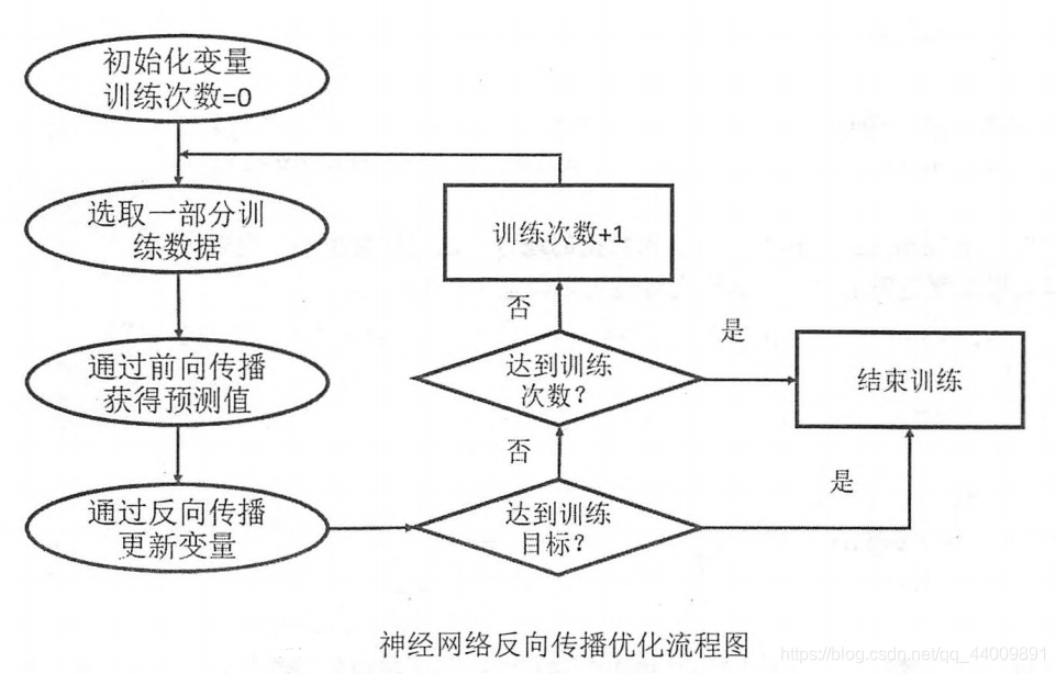
神经网络的优化过程可以分为两个阶段:
-
第一个阶段,通过前向传播算法计算得到预测值,并将预测值和真实值做对比得出两者之间的差距。
计算神经网络的前向传播的结果需要三部分的信息:
-
第一部分是神经网络的输入,这个输入就是从实体中提取的特征向量;
-
第二部分是神经网络的连接结构,即不同神经元之间输入输出的连接关系;
-
第三部分是神经网络中神经元之间的边的权重。
-
-
第二个阶段,通过反向传播算法(backpropagation)计算损失函数对每一个参数的梯度,再根据梯度和学习率使用梯度下降算法(gradient decent)更新每一个参数。通俗的理解就是,梯度下降算法主要用于优化单个参数的取值,而反向传播算法给出了一个高效的方式在所有参数上使用梯度下降算法,从而使神经网络模型在训练数据上的损失函数尽可能小。
反向传播算法是训练神经网络的核心算法,它可以根据定义好的损失函数优化神经网络中参数的取值,从而使神经网络模型在训练数据集上的损失函数达到一个较小值,神经网络模型中参数的优化过程直接决定了模型的质量。
反向传播算法实现了一个迭代的过程:
-
第一步,在每次迭代的开始,都选取一小部分的数据,这一小部分数据叫做一个 batch;
-
第二步,这个 batch 的样本会通过前向传播算法得到神经网络模型的预测结果,因为训练数据都是有真实标签的,所以可以计算当前神经网络模型的预测结果和真实结果的差距即损失函数;
-
第三步,基于预测结果和真实结果的差距,反向传播算法会相应更新神经网络模型参数的取值,使模型的预测结果在这个 batch 上更接近真实结果。
-
根据以上内容,运用前向传播和反向传播,我们可以将之前构造好的各个模块进行组合,来搭建我们的全连接神经网络模型,然后使用梯度下降算法对神经网络的参数进行更新:
W
=
W
+
△
W
=
W
+
(
−
η
∂
L
o
s
s
∂
W
)
W = W + \triangle W = W + (- \eta \frac{\partial Loss}{\partial W})
W=W+△W=W+(−η∂W∂Loss)
# 搭建全连接神经网络模型
class FullConnectionModel():
    def __init__(self, latent_dims):
        self.W1 = np.random.normal(loc=0, scale=1, size=[28 * 28 + 1, latent_dims]) / np.sqrt((28 * 28 + 1) / 2)  # He 初始化,有效提高 Relu 网络的性能
        self.W2 = np.random.normal(loc=0, scale=1, size=[latent_dims, 10]) / np.sqrt(latent_dims / 2)  # He 初始化,有效提高 Relu 网络的性能
        self.mul_h1 = FullConnectionLayer()
        self.relu = Relu()
        self.mul_h2 = FullConnectionLayer()
        self.softmax = Softmax()
        self.cross_en = CrossEntropy()

    def forward(self, X, labels):
        bias = np.ones(shape=[X.shape[0], 1])
        X = np.concatenate([X, bias], axis=1)
        self.h1 = self.mul_h1.forward(X, self.W1)
        self.h1_relu = self.relu.forward(self.h1)
        self.h2 = self.mul_h2.forward(self.h1_relu, self.W2)
        self.h2_soft = self.softmax.forward(self.h2)
        self.loss = self.cross_en.forward(self.h2_soft, labels)

    def backward(self, labels):
        self.loss_grad = self.cross_en.backward(labels)
        self.h2_soft_grad = self.softmax.backward(self.loss_grad)
        self.h2_grad, self.W2_grad = self.mul_h2.backward(self.h2_soft_grad)
        self.h1_relu_grad = self.relu.backward(self.h2_grad)
        self.h1_grad, self.W1_grad = self.mul_h1.backward(self.h1_relu_grad)


# 计算精确度
def computeAccuracy(prob, labels):
    predicitions = np.argmax(prob, axis=1)
    truth = np.argmax(labels, axis=1)
    return np.mean(predicitions == truth)


# 训练一次模型
def trainOneStep(model, x_train, y_train, learning_rate=1e-5):
    model.forward(x_train, y_train)
    model.backward(y_train)
    model.W1 += -learning_rate * model.W1_grad
    model.W2 += -learning_rate * model.W2_grad
    loss = model.loss
    accuracy = computeAccuracy(model.h2_soft, y_train)
    return loss, accuracy


model = FullConnectionModel()
loss, accuracy = trainOneStep(model, mnist.train.images, mnist.train.labels)
上面的程序实现了训练全连接神经网络的过程,从这段程序我们可以总结出训练神经网络的 3 个步骤:
-
第一步,定义神经网络的结构和前向传播的输出结果;
-
第二步,定义损失函数以及选择反向传播优化的算法;
-
第三步,在训练数据上运行反向传播优化算法。
7 模型的训练和评估
到上一步整个全连接神经网络框架基本已经搭建完成了,在这一步我们就可以对模型进行训练和评估了,我们在 1 数据集的下载与处理 已经划分了训练集、验证集和测试集,因此这里我们可以借助验证集进行参数寻优,找出最好的参数组合,然后将由这组参数训练来的模型在测试集上进行测试:
# 训练模型和寻优
def train(x_train, y_train, x_validation, y_validation):
    epochs = 200
    learning_rate = 1e-5
    latent_dims_list = [100, 200, 300]
    best_accuracy = 0
    best_latent_dims = 0

    # 在验证集上寻优
    print("Start seaching the best parameter...\n")
    for latent_dims in latent_dims_list:
        model = FullConnectionModel(latent_dims)

        bar = trange(20)  # 使用 tqdm 第三方库,调用 tqdm.std.trange 方法给循环加个进度条
        for epoch in bar:
            loss, accuracy = trainOneStep(model, x_train, y_train, learning_rate)
            bar.set_description(f'Parameter latent_dims={latent_dims: <3}, epoch={epoch + 1: <3}, loss={loss: <10.8}, accuracy={accuracy: <8.6}')  # 给进度条加个描述
        bar.close()

        validation_loss, validation_accuracy = evaluate(model, x_validation, y_validation)
        print(f"Parameter latent_dims={latent_dims: <3}, validation_loss={validation_loss}, validation_accuracy={validation_accuracy}.\n")

        if validation_accuracy > best_accuracy:
            best_accuracy = validation_accuracy
            best_latent_dims = latent_dims

    # 得到最好的参数组合,训练最好的模型
    print(f"The best parameter is {best_latent_dims}.\n")
    print("Start training the best model...")
    best_model = FullConnectionModel(best_latent_dims)
    x = np.concatenate([x_train, x_validation], axis=0)
    y = np.concatenate([y_train, y_validation], axis=0)
    bar = trange(epochs)
    for epoch in bar:
        loss, accuracy = trainOneStep(best_model, x, y, learning_rate)
        bar.set_description(f'Training the best model, epoch={epoch + 1: <3}, loss={loss: <10.8}, accuracy={accuracy: <8.6}')  # 给进度条加个描述
    bar.close()

    return best_model


# 评估模型
def evaluate(model, x, y):
    model.forward(x, y)
    loss = model.loss
    accuracy = computeAccuracy(model.h2_soft, y)
    return loss, accuracy


mnist = input_data.read_data_sets("dataset/", one_hot=True)
model = train(mnist.train.images, mnist.train.labels, mnist.validation.images, mnist.validation.labels)
loss, accuracy = evaluate(model, mnist.test.images, mnist.test.labels)
print(f'Evaluate the best model, test loss={loss:0<10.8}, accuracy={accuracy:0<8.6}.')
运行上述代码,结果如下,可以看到模型的准确率能够达到 0.94,说明模型的性能还是相当不错的:

8 组合模块形成完整代码
最后,将前面的所有模块进行组合,并添加 main 函数,得到完整代码:
'''
Description: 自己动手写神经网络(一)——初步搭建全连接神经网络框架
Author: stepondust
Date: 2020-12-2
'''
import numpy as np
from tensorflow.examples.tutorials.mnist import input_data
from tqdm._tqdm import trange


# 构造全连接层,实现 X 和 W 的矩阵乘法运算
class FullConnectionLayer():
    def __init__(self):
        self.mem = {}

    def forward(self, X, W):
        '''
        param {
            X: shape(m, d), 前向传播输入矩阵
            W: shape(d, d'), 前向传播权重矩阵
        }
        return {
            H: shape(m, d'), 前向传播输出矩阵
        }
        '''
        self.mem["X"] = X
        self.mem["W"] = W
        H = np.matmul(X, W)
        return H

    def backward(self, grad_H):
        '''
        param {
            grad_H: shape(m, d'), Loss 关于 H 的梯度
        }
        return {
            grad_X: shape(m, d), Loss 关于 X 的梯度
            grad_W: shape(d, d'), Loss 关于 W 的梯度
        }
        '''
        X = self.mem["X"]
        W = self.mem["W"]
        grad_X = np.matmul(grad_H, W.T)
        grad_W = np.matmul(X.T, grad_H)
        return grad_X, grad_W


# 实现 Relu 激活函数
class Relu():
    def __init__(self):
        self.mem = {}

    def forward(self, X):
        self.mem["X"] = X
        return np.where(X > 0, X, np.zeros_like(X))

    def backward(self, grad_y):
        X = self.mem["X"]
        return (X > 0).astype(np.float32) * grad_y


# 实现 Softmax 激活函数
class Softmax():
    def __init__(self):
        self.mem = {}
        self.epsilon = 1e-12  # 防止求导后分母为 0

    def forward(self, p):
        p_exp = np.exp(p)
        denominator = np.sum(p_exp, axis=1, keepdims=True)
        s = p_exp / (denominator + self.epsilon)
        self.mem["s"] = s
        self.mem["p_exp"] = p_exp
        return s

    def backward(self, grad_s):
        s = self.mem["s"]
        sisj = np.matmul(np.expand_dims(s, axis=2), np.expand_dims(s, axis=1))
        tmp = np.matmul(np.expand_dims(grad_s, axis=1), sisj)
        tmp = np.squeeze(tmp, axis=1)
        grad_p = -tmp + grad_s * s
        return grad_p


# 实现交叉熵损失函数
class CrossEntropy():
    def __init__(self):
        self.mem = {}
        self.epsilon = 1e-12  # 防止求导后分母为 0

    def forward(self, p, y):
        self.mem['p'] = p
        log_p = np.log(p + self.epsilon)
        return np.mean(np.sum(-y * log_p, axis=1))

    def backward(self, y):
        p = self.mem['p']
        return -y * (1 / (p + self.epsilon))


# 搭建全连接神经网络模型
class FullConnectionModel():
    def __init__(self, latent_dims):
        self.W1 = np.random.normal(loc=0, scale=1, size=[28 * 28 + 1, latent_dims]) / np.sqrt((28 * 28 + 1) / 2)  # He 初始化,有效提高 Relu 网络的性能
        self.W2 = np.random.normal(loc=0, scale=1, size=[latent_dims, 10]) / np.sqrt(latent_dims / 2)  # He 初始化,有效提高 Relu 网络的性能
        self.mul_h1 = FullConnectionLayer()
        self.relu = Relu()
        self.mul_h2 = FullConnectionLayer()
        self.softmax = Softmax()
        self.cross_en = CrossEntropy()

    def forward(self, X, labels):
        bias = np.ones(shape=[X.shape[0], 1])
        X = np.concatenate([X, bias], axis=1)
        self.h1 = self.mul_h1.forward(X, self.W1)
        self.h1_relu = self.relu.forward(self.h1)
        self.h2 = self.mul_h2.forward(self.h1_relu, self.W2)
        self.h2_soft = self.softmax.forward(self.h2)
        self.loss = self.cross_en.forward(self.h2_soft, labels)

    def backward(self, labels):
        self.loss_grad = self.cross_en.backward(labels)
        self.h2_soft_grad = self.softmax.backward(self.loss_grad)
        self.h2_grad, self.W2_grad = self.mul_h2.backward(self.h2_soft_grad)
        self.h1_relu_grad = self.relu.backward(self.h2_grad)
        self.h1_grad, self.W1_grad = self.mul_h1.backward(self.h1_relu_grad)


# 计算精确度
def computeAccuracy(prob, labels):
    predicitions = np.argmax(prob, axis=1)
    truth = np.argmax(labels, axis=1)
    return np.mean(predicitions == truth)


# 训练一次模型
def trainOneStep(model, x_train, y_train, learning_rate=1e-5):
    model.forward(x_train, y_train)
    model.backward(y_train)
    model.W1 += -learning_rate * model.W1_grad
    model.W2 += -learning_rate * model.W2_grad
    loss = model.loss
    accuracy = computeAccuracy(model.h2_soft, y_train)
    return loss, accuracy


# 训练模型和寻优
def train(x_train, y_train, x_validation, y_validation):
    epochs = 200
    learning_rate = 1e-5
    latent_dims_list = [100, 200, 300]
    best_accuracy = 0
    best_latent_dims = 0

    # 在验证集上寻优
    print("Start seaching the best parameter...\n")
    for latent_dims in latent_dims_list:
        model = FullConnectionModel(latent_dims)

        bar = trange(20)  # 使用 tqdm 第三方库,调用 tqdm.std.trange 方法给循环加个进度条
        for epoch in bar:
            loss, accuracy = trainOneStep(model, x_train, y_train, learning_rate)
            bar.set_description(f'Parameter latent_dims={latent_dims: <3}, epoch={epoch + 1: <3}, loss={loss: <10.8}, accuracy={accuracy: <8.6}')  # 给进度条加个描述
        bar.close()

        validation_loss, validation_accuracy = evaluate(model, x_validation, y_validation)
        print(f"Parameter latent_dims={latent_dims: <3}, validation_loss={validation_loss}, validation_accuracy={validation_accuracy}.\n")

        if validation_accuracy > best_accuracy:
            best_accuracy = validation_accuracy
            best_latent_dims = latent_dims

    # 得到最好的参数组合,训练最好的模型
    print(f"The best parameter is {best_latent_dims}.\n")
    print("Start training the best model...")
    best_model = FullConnectionModel(best_latent_dims)
    x = np.concatenate([x_train, x_validation], axis=0)
    y = np.concatenate([y_train, y_validation], axis=0)
    bar = trange(epochs)
    for epoch in bar:
        loss, accuracy = trainOneStep(best_model, x, y, learning_rate)
        bar.set_description(f'Training the best model, epoch={epoch + 1: <3}, loss={loss: <10.8}, accuracy={accuracy: <8.6}')  # 给进度条加个描述
    bar.close()

    return best_model


# 评估模型
def evaluate(model, x, y):
    model.forward(x, y)
    loss = model.loss
    accuracy = computeAccuracy(model.h2_soft, y)
    return loss, accuracy


if __name__ == '__main__':
    mnist = input_data.read_data_sets("dataset/", one_hot=True)

    model = train(mnist.train.images, mnist.train.labels, mnist.validation.images, mnist.validation.labels)

    loss, accuracy = evaluate(model, mnist.test.images, mnist.test.labels)
    print(f'Evaluate the best model, test loss={loss:0<10.8}, accuracy={accuracy:0<8.6}.')
好了本文到此就快结束了,以上就是我自己动手写全连接神经网络的想法和思路,大家参照一下即可,重要的还是经过自己的思考来编写代码,文章中还有很多不足和不正确的地方,欢迎大家指正(也请大家体谅,写一篇博客真的挺累的,花的时间比我写出代码的时间还要长),我会尽快修改,之后我也会尽量完善本文,尽量写得通俗易懂。
博文创作不易,转载请注明本文地址:https://blog.csdn.net/qq_44009891/article/details/110475333


 7960
7960


 被折叠的 条评论
为什么被折叠?
被折叠的 条评论
为什么被折叠?
 到【灌水乐园】发言


