动手实现标签传播--LP-simple-example

from IPython.display import set_matplotlib_formats
%matplotlib inline
#set_matplotlib_formats('svg', 'pdf')
 
import numpy as np
import pandas as pd
import matplotlib.pyplot as plt
from scipy.spatial.distance import cdist
from sklearn.datasets import make_moons
 
 # save_dir = '../data/images' 存储位置 怎么看？？？？？？？？

一：创建一个简单的数据集

n = 800   # 样本数
n_labeled = 10 # 有标签样本数
X, Y = make_moons(n, shuffle=True, noise=0.1, random_state=1000)
 
X.shape, Y.shape

((800, 2), (800,))

def one_hot(Y, n_classes):
    '''
    对标签做 one_hot 编码
    
    参数
    =====
    Y: 从 0 开始的标签
    n_classes: 类别数
    '''
    out = Y[:, None] == np.arange(n_classes)
    return out.astype(float)

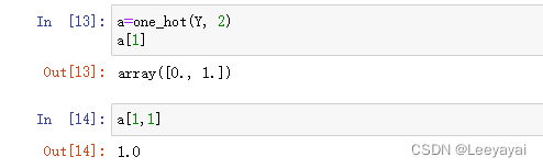
type(one_hot(Y, 2))

numpy.ndarray

# pandas数据，head（10）查看前10条数据
# one_hot(Y, 2).head(10)
# numpy.ndarray没有.head(10)的属性
# ndarray 数组类型--对比matlab里的数据查看，list数据查看

!

查看数据直接用索引

color = ['red' if l == 0 else 'blue' for l in Y]
plt.scatter(X[:, 0], X[:, 1], color=color)
#plt.savefig(f"{save_dir}/bi_classification.pdf", format='pdf')  存储位置怎么看？？？
plt.show()
 
Y_input = np.concatenate((one_hot(Y[:n_labeled], 2), 
                          np.zeros((n-n_labeled, 2))))
# np.concatenate()用以数组拼接，如上拼接2维的标签矩阵Y与2维0矩阵（800*2）
# 拼接后数据，800*2，1600个？？
# np.zeros((n-n_labeled, 2)) 生成一个n-n_labeled*2的0矩阵
# 前面有样本的标签数，10个标签，Y的

二：算法过程

Step 1: 创建相似度矩阵 W

def rbf(x, sigma):
    return np.exp((-x)/(2* sigma**2))

sigma = 0.2
dm = cdist(X, X, 'euclidean')
W = rbf(dm, sigma)
np.fill_diagonal(W, 0)   # 对角线全为 0
print(W)
print(dm)

[[0.00000000e+00 6.88881737e-13 1.21765707e-10 ... 1.13529410e-07
  2.11124727e-08 5.46799123e-12]
 [6.88881737e-13 0.00000000e+00 2.26817428e-05 ... 5.38938664e-06
  7.13302960e-09 1.24874906e-01]
 [1.21765707e-10 2.26817428e-05 0.00000000e+00 ... 1.73540864e-05
  1.76781880e-04 6.21313160e-05]
 ...
 [1.13529410e-07 5.38938664e-06 1.73540864e-05 ... 0.00000000e+00
  1.87181241e-06 4.31430874e-05]
 [2.11124727e-08 7.13302960e-09 1.76781880e-04 ... 1.87181241e-06
  0.00000000e+00 3.04407484e-08]
 [5.46799123e-12 1.24874906e-01 6.21313160e-05 ... 4.31430874e-05
  3.04407484e-08 0.00000000e+00]]
[[0.         2.24029654 1.82631379 ... 1.27929631 1.41387215 2.07456878]
 [2.24029654 0.         0.85551602 ... 0.97048632 1.50068238 0.16643542]
 [1.82631379 0.85551602 0.         ... 0.8769346  0.69124751 0.77490083]
 ...
 [1.27929631 0.97048632 0.8769346  ... 0.         1.05508827 0.80407907]
 [1.41387215 1.50068238 0.69124751 ... 1.05508827 0.         1.3845987 ]
 [2.07456878 0.16643542 0.77490083 ... 0.80407907 1.3845987  0.        ]]

Step 2: 计算 S

def calculate_S(W):
    d = np.sum(W, axis=1) 
    D_ = np.sqrt(d*d[:, np.newaxis]) # D_ 是 np.sqrt(np.dot(diag(D),diag(D)^T))
    return np.divide(W, D_, where=D_ != 0)
 
 
S = calculate_S(W)
S ### 权重很小--超参数要设置很小？？

array([[0.00000000e+00, 9.64552480e-14, 1.46510478e-11, ...,
        1.31030774e-08, 2.81050663e-09, 6.69687811e-13],
       [9.64552480e-14, 0.00000000e+00, 2.32394909e-06, ...,
        5.29676568e-07, 8.08585661e-10, 1.30234562e-02],
       [1.46510478e-11, 2.32394909e-06, 0.00000000e+00, ...,
        1.46566824e-06, 1.72207578e-05, 5.56831938e-06],
       ...,
       [1.31030774e-08, 5.29676568e-07, 1.46566824e-06, ...,
        0.00000000e+00, 1.74903325e-07, 3.70890778e-06],
       [2.81050663e-09, 8.08585661e-10, 1.72207578e-05, ...,
        1.74903325e-07, 0.00000000e+00, 3.01835787e-09],
       [6.69687811e-13, 1.30234562e-02, 5.56831938e-06, ...,
        3.70890778e-06, 3.01835787e-09, 0.00000000e+00]])

迭代一次的结果

alpha = 0.99
F = np.dot(S, Y_input)*alpha + (1-alpha)*Y_input  #迭代过程
 
Y_result = np.zeros_like(F)
Y_result[np.arange(len(F)), F.argmax(1)] = 1
 
Y_v = [1 if x == 0 else 0 for x in Y_result[0:,0]]
 
color = ['red' if l == 0 else 'blue' for l in Y_v]
plt.scatter(X[0:,0], X[0:,1], color=color)
#plt.savefig("iter_1.pdf", format='pdf')
plt.show()

Step 3: 迭代 F “n_iter” 次直到收敛

n_iter = 150
F = Y_input
for t in range(n_iter):
    F = np.dot(S, F)*alpha + (1-alpha)*Y_input

Step 4: 画出最终结果

Y_result = np.zeros_like(F)
Y_result[np.arange(len(F)), F.argmax(1)] = 1
 
Y_v = [1 if x == 0 else 0 for x in Y_result[0:,0]]
 
color = ['red' if l == 0 else 'blue' for l in Y_v]
plt.scatter(X[0:,0], X[0:,1], color=color)
#plt.savefig("iter_n.pdf", format='pdf')
plt.show()

from sklearn import metrics
 
print(metrics.classification_report(Y, F.argmax(1)))
 
acc = metrics.accuracy_score(Y, F.argmax(1))
print('准确度为',acc)

              precision    recall  f1-score   support

           0       1.00      0.86      0.92       400
           1       0.88      1.00      0.93       400

    accuracy                           0.93       800
   macro avg       0.94      0.93      0.93       800
weighted avg       0.94      0.93      0.93       800

准确度为 0.92875