


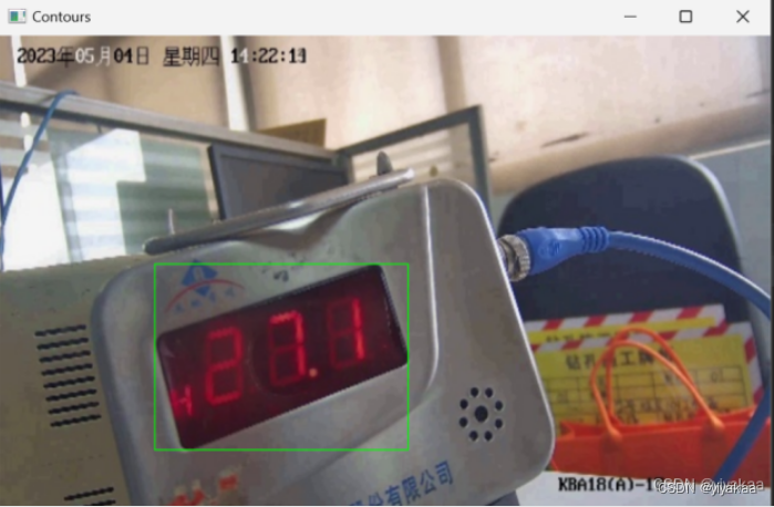
应项目要求需要基于cpu的LED数字识别,为了满足需求,使用传统方法进行实验。识别传感器中显示的数字。因此使用opencv的函数做一些处理,实现功能需求。
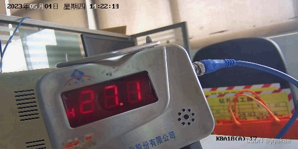
首先读取图像,因为我没想大致得到LED屏幕的区域,因此将RGB转换为HSV空间,并分别设置H、S和V的阈值,让该区域显现出来。可以看到代码中进行了resize操作,这个操作不是必须的,具体H、S和V的数值根据具体的图像自行设置。
img = cv2.imread('pic.jpg')
#start = time.time()
new_size = (640, 400)
img = cv2.resize(img, new_size)
hsv_img = cv2.cvtColor(img, cv2.COLOR_BGR2HSV)
mask = np.zeros(hsv_img.shape[:2], dtype=np.uint8)
mask[(hsv_img[:,:,0] >= 130) & (hsv_img[:,:,0] <= 255) & (hsv_img[:,:,1] >= 0) &
(hsv_img[:,:,1] <= 255) & (hsv_img[:,:,2] >= 0) & (hsv_img[:,:,2] <= 90)] = 1
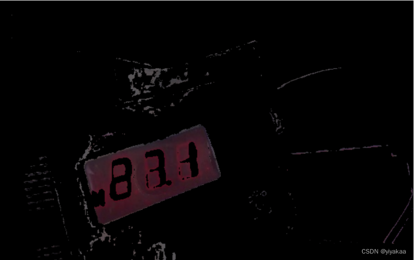
result = cv2.bitwise_and(img, img, mask=mask)
原图处理后结果:
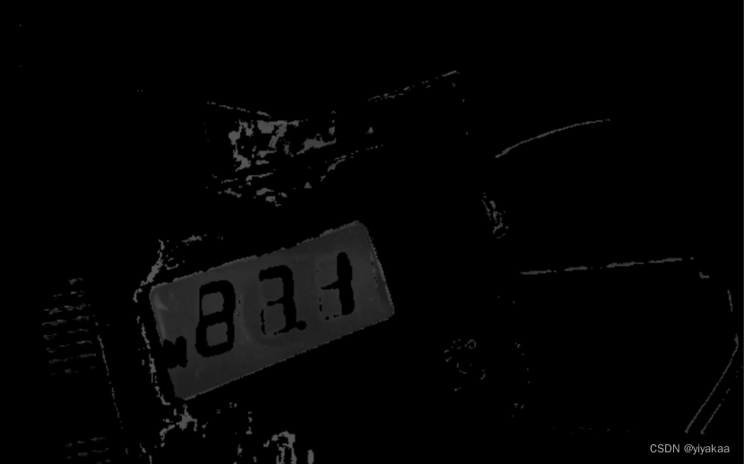
接下来需要检测轮廓信息,因此进行灰度化处理。
gray = cv2.cvtColor(result,cv2.COLOR_BGR2GRAY)
处理后结果:
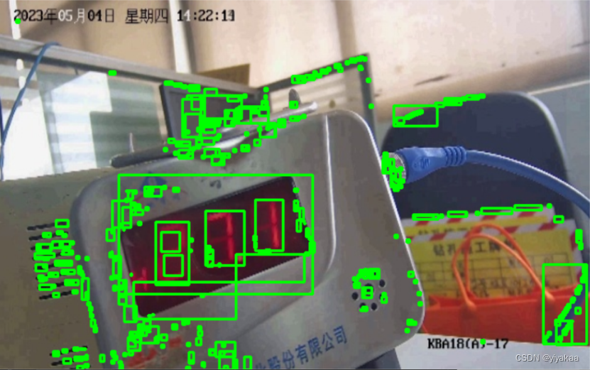
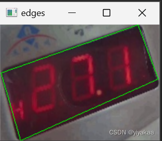
使用Canny做轮廓检测,并保存所有轮廓信息,将所有轮廓信息框选出来,因为框选区域矩形,所以采用面积策略删掉小块区域面积只显示大块的面积。
#转灰度,做单通道计算比较节省时间
edges = cv2.Canny(gray,50,150,apertureSize = 3)
#所有轮廓的列表contours和分层信息
contours, hierarchy = cv2.findContours(edges, cv2.RETR_TREE, cv2.CHAIN_APPROX_SIMPLE)
# print("轮廓数量:", len(contours))
img_copy = img.copy() # 复制原图,避免在原图上直接画框
for cnt in contours:
x, y, w, h = cv2.boundingRect(cnt) # 获取轮廓的边界矩形
area = w * h
if area > 10000:
x, y, w, h = cv2.boundingRect(cnt)
area = w * h
# print("xywh", x, y, w, h)
# print("矩形面积:", area)
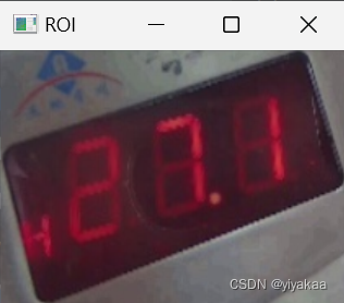
roi = img_copy[y:y + h + 26, x:x + w+2]
# cv2.imshow("ROI", roi)
# cv2.waitKey(0)
# print("矩形面积:", area)
该图为框选的所有轮廓
做面积阈值处理后得到液晶屏幕区域的矩形框:
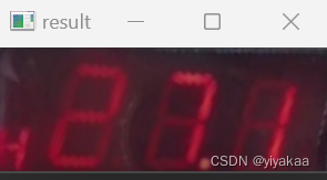
后边拿出框选的区域做处理就行了,直接从原图中拿出框选区域做灰度处理,并作边缘检测,边缘检测前做高斯处理,去除一下噪声。
gray = cv2.cvtColor(roi, cv2.COLOR_BGR2GRAY)
# 高斯滤波
blur = cv2.GaussianBlur(gray, (3, 3), 0)

# 边缘检测
edges = cv2.Canny(gray, 50, 255)
得到框选区域并进行边缘检测结果:
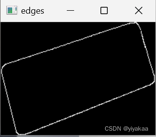
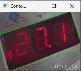
到这里已经检测到LED屏的轮廓了,可以看出我们的拍摄得到的框是斜的,因此需要进行透视校正,而透视校正需要得到四个顶点的坐标值,这里我尝试了两种方法:一、绘制最小外接矩形;二、获取白色像素点坐标(这里自己思考的一种策略,分别按照x轴和y轴找,分别找x轴白色边缘最小值和最大值坐标,y轴白色边缘最小值和最大值坐标)
一、使用最小外接矩形做透视校正
# 获得轮廓信息
contours, hierarchy = cv2.findContours(edges, cv2.RETR_TREE, cv2.CHAIN_APPROX_SIMPLE)

# 绘制最小外接矩形
for cnt in contours:
    rect = cv2.minAreaRect(cnt)
    box = cv2.boxPoints(rect)
    box = np.int0(box)

    cv2.drawContours(roi, [box], 0, (0, 255, 0), 1)

    # 获取矩形的四个顶点坐标
    rect_points = np.int0(cv2.boxPoints(rect))
    # print("矩形的四个顶点坐标:", rect_points)

# cv2.imshow('Contours', roi)
# cv2.waitKey(0)

# 定义原图像的四个角点坐标
src = np.float32([[-8,61],[186 , -3],[ 23, 156], [218 , 91]])

# 定义输出图像的四个角点坐标
dst = np.float32([[0, 0],[200, 0],[0, 100],[200, 100]])

# 计算变换矩阵
M = cv2.getPerspectiveTransform(src, dst)

# 应用变换矩阵
result = cv2.warpPerspective(roi, M, (200, 100))


显示图像
cv2.imshow('Contours', result)
cv2.waitKey(0)
得到最小外接矩形:
透视校正结果:

从最小外接矩形可以看出框选的区域除了LED屏幕还有一些其他区域影响,这边后边的实验中发现,这些多余地方会影响后序的实验准确性。
二、分别获取x轴和y轴白色像素点坐标
# 获取白色像素点坐标
coordinates = np.column_stack(np.where(edges == 255))

# # 打印白色像素点坐标
# print(coordinates)

# 在x轴方向上找到最小和最大的两个坐标
x_min = coordinates[np.argmin(coordinates[:,0])].copy()
x_min[0], x_min[1] = x_min[1], x_min[0]
x_max = coordinates[np.argmax(coordinates[:,0])].copy()
x_max[0], x_max[1] = x_max[1], x_max[0]

# 在y轴方向上找到最小和最大的两个坐标
y_min = coordinates[np.argmin(coordinates[:,1])].copy()
y_min[0], y_min[1] = y_min[1], y_min[0]
y_max = coordinates[np.argmax(coordinates[:,1])].copy()
y_max[0], y_max[1] = y_max[1], y_max[0]

# # # 打印最小和最大的两个坐标
# print('x_min:', x_min)
# print('x_max:', x_max)
# print('y_min:', y_min)
# print('y_max:', y_max)


# 定义原图像的四个角点坐标
src = np.float32([y_min,x_min,x_max, y_max])

# 定义输出图像的四个角点坐标
dst = np.float32([[0, 0],[200, 0],[0, 100],[200, 100]])

# 计算变换矩阵
M = cv2.getPerspectiveTransform(src, dst)

# 应用变换矩阵
result = cv2.warpPerspective(roi, M, (200, 100))
#显示图像
# cv2.imshow('result', result)
# cv2.waitKey(0)
按照思路找x轴和y轴最大最小值对于的白色像素点坐标并绘制框:
透视校正后:
将透视校正后的图像区域继续进行RGB转换HSV,并设置阈值使数字区域更好的显示出来
hsv_img = cv2.cvtColor(result, cv2.COLOR_BGR2HSV)
# cv2.imshow('hsv_img', hsv_img)
# cv2.waitKey(0)
mask = np.zeros(hsv_img.shape[:2], dtype=np.uint8)
mask[(hsv_img[:,:,0] >= 0) & (hsv_img[:,:,0] <= 255) & (hsv_img[:,:,1] >= 0) &
(hsv_img[:,:,1] <= 255) & (hsv_img[:,:,2] >= 0) & (hsv_img[:,:,2] <= 100)] = 1
result1 = cv2.bitwise_and(hsv_img, hsv_img, mask=mask)

# cv2.imshow("Contours", result1)
# cv2.waitKey(0)
RGB转换HSV:
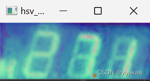
H、S和V设置阈值使数字区域显示:
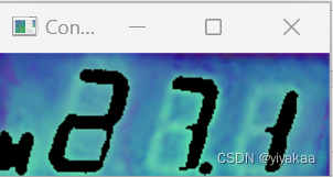
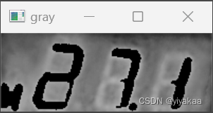
将得到的图像进行二值化处理
# 转换为灰度图像
gray = cv2.cvtColor(result1, cv2.COLOR_BGR2GRAY)
# cv2.imshow('gray', gray)
# cv2.waitKey(0)
#
#二值化处理
_, binary = cv2.threshold(gray, 50, 255, cv2.THRESH_BINARY)

#
# cv2.imshow("Contours", binary)
# cv2.waitKey(0)
灰度处理和二值化后的结果:
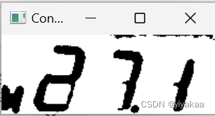
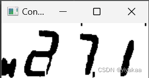
可以看到图像中含有多余的部分,继续使用形态学操作(腐蚀)处理。这里分别进行x方向和y方向的腐蚀操作。
# 自定义 1x3 的核进行 x 方向的膨胀腐蚀
kernel = cv2.getStructuringElement(cv2.MORPH_RECT, (1, 3))
xtx_img = cv2.dilate(binary, kernel, iterations=3)
xtx_img = cv2.erode(xtx_img, kernel, iterations=3)#y 腐蚀去除碎片

# cv2.imshow("Contours", xtx_img)
# cv2.waitKey(0)

# 自定义 3x1 的核进行 y 方向的膨胀腐蚀
kernel = cv2.getStructuringElement(cv2.MORPH_RECT, (3, 1))
xtx_img = cv2.dilate(xtx_img, kernel, iterations=3)#x 膨胀回复形态
xtx_img = cv2.erode(xtx_img, kernel, iterations=3)#x 腐蚀去除碎片
#
# cv2.imshow("Contours", xtx_img)
# cv2.waitKey(0)
x方向腐蚀结果:
y方向腐蚀结果
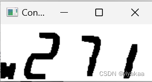
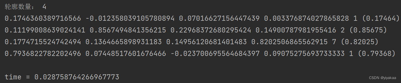
然后需要找到所有的轮廓,因为opencv中默认函数找到的是白色轮廓,因此需要将得到的二值化结果取反操作。再使用函数获取所有的白色轮廓。运行出来的结果符合预期,确实是4。
# 将二值化图像取反
binary_inv = cv2.bitwise_not(xtx_img)
# cv2.imshow("Contours", binary_inv)
# cv2.waitKey(0)
#所有轮廓的列表contours和分层信息
contours, hierarchy = cv2.findContours(binary_inv, cv2.RETR_TREE, cv2.CHAIN_APPROX_SIMPLE)

# 打印轮廓数量

print("轮廓数量:", len(contours))
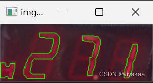
得到轮廓后绘制在原图上看一下
img_contour = cv2.drawContours(result, contours, -1, (0, 255, 0), 1)

# cv2.imshow("img_contour", img_contour)
# cv2.waitKey(0)
感觉像那么回事了:
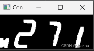
得到轮廓后按照轮廓的x轴坐标进行排序,以免后序识别中顺序乱了,从这每个数字就被我们单独拿出来了。
# 存储所有轮廓的图像
plate_imgs = []

# 获取所有轮廓的x坐标
x_coordinates = []
for contour in contours:
    x, y, w, h = cv2.boundingRect(contour)
    x_coordinates.append(x)

# 将轮廓按照x坐标排序
sorted_contours = [contours[i] for i in np.argsort(x_coordinates)]
有了这些数字后,就需要分别识别这些数字都是数字几了,这里可以使用分类任务,训练一个自己的模型识别这些数字,这里我们采用一种自己研究生方向学到的结构相似性来做识别,只要能识别出来就行,结构相似性的值在0-1之间,越大说明两个图像越像(大概可以这么理解),因此我们提前保存好数字的图片,并且图片的名字分别对应数字的编号,这样在识别出来后,就直接打印图片的命名就知道这个数字是几了,因为这个LED屏幕中只有2、7、1三个数字因此我们只保存了这三张图片,用来识别,至于前边的第一个框区域不识别,是因为除过这些数字外还有CO甲烷等东西,这里没有做识别。我们分别将分割出来的每个数字和提前保存到文件夹中的数字对比结构相似性,保留结构相似性最高的数字以及文件名最终得到识别结果。
# 初始化最高相似度和对应文件名
max_sim = -1
max_sim_filename = ''

# 按x轴逐个绘制
for i, contour in enumerate(sorted_contours):
    x, y, w, h = cv2.boundingRect(contour)
    cv2.rectangle(xtx_img, (x, y), (x + w, y + h), (0, 255, 0), 1)
    plate_img1 = binary_inv[y:y + h, x:x + w].copy()
    # 生成文件名,加上时间戳
    # filename = f"saved_image_{i}_{int(time.time())}.jpg"
    # cv2.imwrite(filename, plate_img1)
    # cv2.imshow("img_contour", plate_img1)
    # cv2.waitKey(0)
    plate_img = cv2.resize(plate_img1, (22, 60))
    # cv2.imshow("img_contour", plate_img)
    # cv2.waitKey(0)

    max_sim = 0
    # 遍历result文件夹下的所有文件
    for filename in os.listdir('Desktop\\count\\result2'):
        if filename.endswith('.png'):
            # 读取图像并resize//C:\\Users\\12561\\Desktop\\count\\result\\
            img2 = cv2.imread(os.path.join('Desktop\\count\\result2', filename), cv2.IMREAD_GRAYSCALE)
            img2 = cv2.resize(img2, (22, 60))

            # 计算相似度
            similarity = ssim(plate_img, img2)
            print(similarity, end=' ')
            # 如果相似度更高,则更新最高相似度和对应文件名
            if similarity > max_sim:
                max_sim = similarity
                max_sim_filename = os.path.splitext(filename)[0]  # 去掉文件后缀
    #if max_sim_filename == '_':
        #max_sim_filename = '.'
    # print(max_sim_filename, end='')
    print(f"{max_sim_filename} ({max_sim:.5f})", end=' ')
    print()
最终运行结果打印了每种图像的结构相似性值,得到最大的,并且处理速度很快,完全可以在CPU下实现快速处理。
项目完整代码:
import cv2
import numpy as np
import time
import os
from skimage.metrics import structural_similarity as ssim


img = cv2.imread('304.jpg')
start = time.time()
new_size = (640, 400)
img = cv2.resize(img, new_size)
hsv_img = cv2.cvtColor(img, cv2.COLOR_BGR2HSV)
mask = np.zeros(hsv_img.shape[:2], dtype=np.uint8)
mask[(hsv_img[:,:,0] >= 130) & (hsv_img[:,:,0] <= 255) & (hsv_img[:,:,1] >= 0) &
(hsv_img[:,:,1] <= 255) & (hsv_img[:,:,2] >= 0) & (hsv_img[:,:,2] <= 90)] = 1
result = cv2.bitwise_and(img, img, mask=mask)

# cv2.imshow("Contours", result)
# cv2.waitKey(0)

gray = cv2.cvtColor(result,cv2.COLOR_BGR2GRAY)

# cv2.imshow("Contours", gray)
# cv2.waitKey(0)


#边缘检测
#转灰度,做单通道计算比较节省时间
edges = cv2.Canny(gray,50,150,apertureSize = 3)

#所有轮廓的列表contours和分层信息
contours, hierarchy = cv2.findContours(edges, cv2.RETR_TREE, cv2.CHAIN_APPROX_SIMPLE)
# print("轮廓数量:", len(contours))

img_copy = img.copy() # 复制原图,避免在原图上直接画框

for cnt in contours:
    x, y, w, h = cv2.boundingRect(cnt) # 获取轮廓的边界矩形
    area = w * h
    if area > 10000:
        x, y, w, h = cv2.boundingRect(cnt)
        area = w * h
        # print("xywh", x, y, w, h)
        # print("矩形面积:", area)
        roi = img_copy[y:y + h + 26, x:x + w+2]
        # cv2.imshow("ROI", roi)
        # cv2.waitKey(0)
        # print("矩形面积:", area)
        # cv2.rectangle(img_copy, (x, y), (x + w, y + h + 25), (0, 255, 0), 1)  # 画矩形框,绿色,宽度为2

# cv2.imshow("ROI", roi)
# cv2.waitKey(0)

# 转换为灰度图像
gray = cv2.cvtColor(roi, cv2.COLOR_BGR2GRAY)
# 高斯滤波
blur = cv2.GaussianBlur(gray, (3, 3), 0)

# 边缘检测
edges = cv2.Canny(gray, 50, 255)
# cv2.imshow("ROI", edges)
# cv2.waitKey(0)

# # 获得轮廓信息
# contours, hierarchy = cv2.findContours(edges, cv2.RETR_TREE, cv2.CHAIN_APPROX_SIMPLE)
#
# # 绘制最小外接矩形
# for cnt in contours:
#     rect = cv2.minAreaRect(cnt)
#     box = cv2.boxPoints(rect)
#     box = np.int0(box)
#
#     cv2.drawContours(roi, [box], 0, (0, 255, 0), 1)
#
#     # 获取矩形的四个顶点坐标
#     rect_points = np.int0(cv2.boxPoints(rect))
#     # print("矩形的四个顶点坐标:", rect_points)
#
# # cv2.imshow('Contours', roi)
# # cv2.waitKey(0)
#
# # 定义原图像的四个角点坐标
# src = np.float32([[-8,61],[186 , -3],[ 23, 156], [218 , 91]])
#
# # 定义输出图像的四个角点坐标
# dst = np.float32([[0, 0],[200, 0],[0, 100],[200, 100]])
#
# # 计算变换矩阵
# M = cv2.getPerspectiveTransform(src, dst)
#
# # 应用变换矩阵
# result = cv2.warpPerspective(roi, M, (200, 100))
#
#
# 显示图像
# cv2.imshow('Contours', result)
# cv2.waitKey(0)

#
# 获取白色像素点坐标
coordinates = np.column_stack(np.where(edges == 255))

# # 打印白色像素点坐标
# print(coordinates)

# 在x轴方向上找到最小和最大的两个坐标
x_min = coordinates[np.argmin(coordinates[:,0])].copy()
x_min[0], x_min[1] = x_min[1], x_min[0]
x_max = coordinates[np.argmax(coordinates[:,0])].copy()
x_max[0], x_max[1] = x_max[1], x_max[0]

# 在y轴方向上找到最小和最大的两个坐标
y_min = coordinates[np.argmin(coordinates[:,1])].copy()
y_min[0], y_min[1] = y_min[1], y_min[0]
y_max = coordinates[np.argmax(coordinates[:,1])].copy()
y_max[0], y_max[1] = y_max[1], y_max[0]

# # # 打印最小和最大的两个坐标
# print('x_min:', x_min)
# print('x_max:', x_max)
# print('y_min:', y_min)
# print('y_max:', y_max)


# 定义原图像的四个角点坐标
src = np.float32([y_min,x_min,x_max, y_max])

# 定义输出图像的四个角点坐标
dst = np.float32([[0, 0],[200, 0],[0, 100],[200, 75]])

# 计算变换矩阵
M = cv2.getPerspectiveTransform(src, dst)

# 应用变换矩阵
result = cv2.warpPerspective(roi, M, (200, 75))
#显示图像
# cv2.imshow('result', result)
# cv2.waitKey(0)

# gray = cv2.cvtColor(result, cv2.COLOR_BGR2GRAY)
# cv2.imshow('hsv_img', gray)
# cv2.waitKey(0)

hsv_img = cv2.cvtColor(result, cv2.COLOR_BGR2HSV)
# cv2.imshow('hsv_img', hsv_img)
# cv2.waitKey(0)
mask = np.zeros(hsv_img.shape[:2], dtype=np.uint8)
mask[(hsv_img[:,:,0] >= 0) & (hsv_img[:,:,0] <= 255) & (hsv_img[:,:,1] >= 0) &
(hsv_img[:,:,1] <= 255) & (hsv_img[:,:,2] >= 0) & (hsv_img[:,:,2] <= 100)] = 1
result1 = cv2.bitwise_and(hsv_img, hsv_img, mask=mask)

# cv2.imshow("Contours", result1)
# cv2.waitKey(0)

# 转换为灰度图像
gray = cv2.cvtColor(result1, cv2.COLOR_BGR2GRAY)
# cv2.imshow('gray', gray)
# cv2.waitKey(0)
#
#二值化处理
_, binary = cv2.threshold(gray, 50, 255, cv2.THRESH_BINARY)

#
# cv2.imshow("Contours", binary)
# cv2.waitKey(0)

# 自定义 1x3 的核进行 x 方向的膨胀腐蚀
kernel = cv2.getStructuringElement(cv2.MORPH_RECT, (1, 3))
xtx_img = cv2.dilate(binary, kernel, iterations=3)
xtx_img = cv2.erode(xtx_img, kernel, iterations=3)#y 腐蚀去除碎片

# cv2.imshow("Contours", xtx_img)
# cv2.waitKey(0)

# 自定义 3x1 的核进行 y 方向的膨胀腐蚀
kernel = cv2.getStructuringElement(cv2.MORPH_RECT, (3, 1))
xtx_img = cv2.dilate(xtx_img, kernel, iterations=3)#x 膨胀回复形态
xtx_img = cv2.erode(xtx_img, kernel, iterations=3)#x 腐蚀去除碎片
#
# cv2.imshow("Contours", xtx_img)
# cv2.waitKey(0)

# 将二值化图像取反
binary_inv = cv2.bitwise_not(xtx_img)
# cv2.imshow("Contours", binary_inv)
# cv2.waitKey(0)
#所有轮廓的列表contours和分层信息
contours, hierarchy = cv2.findContours(binary_inv, cv2.RETR_TREE, cv2.CHAIN_APPROX_SIMPLE)

# 打印轮廓数量

print("轮廓数量:", len(contours))

# # 创建一个空图像,与原图像大小和通道数相同
# contours_img = np.zeros_like(result)

# 绘制轮廓
img_contour = cv2.drawContours(result, contours, -1, (0, 255, 0), 1)

# cv2.imshow("img_contour", img_contour)
# cv2.waitKey(0)

# 存储所有轮廓的图像
plate_imgs = []

# 获取所有轮廓的x坐标
x_coordinates = []
for contour in contours:
    x, y, w, h = cv2.boundingRect(contour)
    x_coordinates.append(x)

# 将轮廓按照x坐标排序
sorted_contours = [contours[i] for i in np.argsort(x_coordinates)]

# 初始化最高相似度和对应文件名
max_sim = -1
max_sim_filename = ''

# 按x轴逐个绘制
for i, contour in enumerate(sorted_contours):
    x, y, w, h = cv2.boundingRect(contour)
    cv2.rectangle(xtx_img, (x, y), (x + w, y + h), (0, 255, 0), 1)
    plate_img1 = binary_inv[y:y + h, x:x + w].copy()
    # 生成文件名,加上时间戳
    # filename = f"saved_image_{i}_{int(time.time())}.jpg"
    # cv2.imwrite(filename, plate_img1)
    # cv2.imshow("img_contour", plate_img1)
    # cv2.waitKey(0)
    plate_img = cv2.resize(plate_img1, (22, 60))
    # cv2.imshow("img_contour", plate_img)
    # cv2.waitKey(0)

    max_sim = 0
    # 遍历result文件夹下的所有文件
    for filename in os.listdir('Desktop\\count\\result2'):
        if filename.endswith('.png'):
            # 读取图像并resize//C:\\Users\\12561\\Desktop\\count\\result\\
            img2 = cv2.imread(os.path.join('Desktop\\count\\result2', filename), cv2.IMREAD_GRAYSCALE)
            img2 = cv2.resize(img2, (22, 60))

            # 计算相似度
            similarity = ssim(plate_img, img2)
            print(similarity, end=' ')
            # 如果相似度更高,则更新最高相似度和对应文件名
            if similarity > max_sim:
                max_sim = similarity
                max_sim_filename = os.path.splitext(filename)[0]  # 去掉文件后缀
    if max_sim_filename == '_':
        max_sim_filename = '.'
    # print(max_sim_filename, end='')
    print(f"{max_sim_filename} ({max_sim:.5f})", end=' ')
    print()
    # print(max_sim_filename)
    # cv2.imwrite("C:\\Users\\12561\\Desktop\\count\\result\\plate_img1.png", dilation)  # 保存结果为 PNG 文件
    # cv2.imshow("Contours", plate_img1)
    # cv2.waitKey(0)

print()
end = time.time();
print("time =",end-start)
项目中很多阈值都需要按照特殊图片特殊设置。
总体步骤:
- 轮廓检测
- 透视校正
- 字符分割
- 字符识别


 1万+
1万+


 被折叠的 条评论
为什么被折叠?
被折叠的 条评论
为什么被折叠?
 到【灌水乐园】发言


