吴恩达机器学习 ex2 逻辑回归及过拟合 python实现

1 Logistic Regression

	在这个部分你将建立一个基于两次考试成绩来预测学生是否会被大学录取的模型。
	我们将会有之前的申请者的数据作为训练集。

1.1 visualizing the data

	数据的可视化在后期判断使用什么算法时是非常有用的。

可惜的是，我还是对数据可视化有一点摸不着头脑，复杂一点的图就搞不懂了，所以接下来会更新一些matplotlib的学习笔记~大家如果有需要可以跟着我一起学习哦！

这边由于是完成作业，我会先分析吴恩达给出的图上有的图示要求~

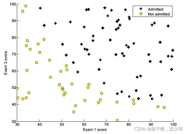
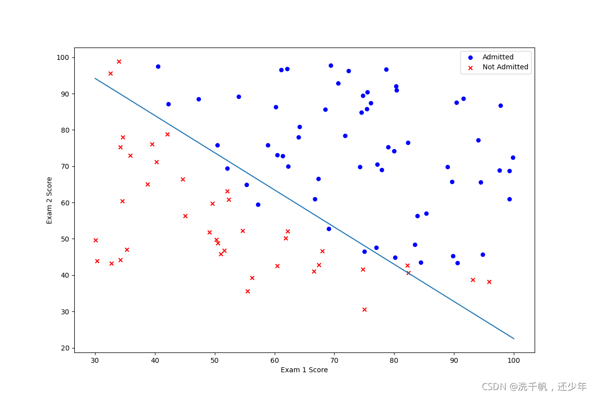
可以看到它的图示区分是按照录取和未录取的~
所以我们需要先对数据区分开录取的和未录取的~（区分正负样本）

path = 'ex2data1.txt'
data = pd.read_csv(path,header=None,names=['Exam 1','Exam s2','Admitted'])

print(data.head())
# 初步预览数据~

positive = data[data['Admitted'].isin([1])]
# isin(values)来查看参数values是否在Series/Data Frame里边，是的话就返回按DataFrame分布布尔值True，否则False
# 此时data['Admitted'].isin([1])是筛选条件
# 而positive才是满足筛选条件的数据
negative = data[data['Admitted'].isin([0])]

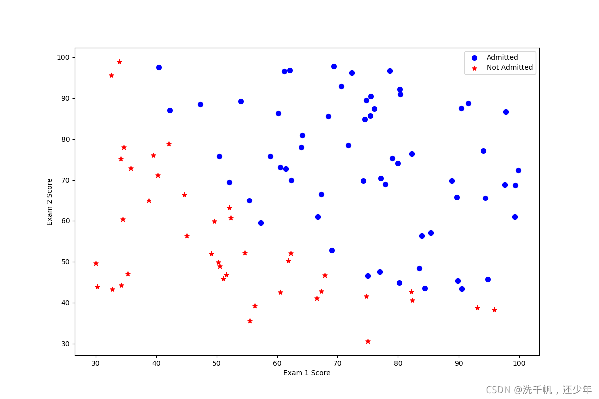
fig,ax = plt.subplots(figsize=(12,8))
ax.scatter(positive['Exam 1'],positive['Exam 2'],s=50,c='b',marker='o',label='Admitted')
# marker='o' 即圈的形状
ax.scatter(negative['Exam 1'],negative['Exam 2'],s=50,c='r',marker='*',label='Not Admitted')
# *用星号表示negative
ax.legend()
ax.set_xlabel('Exam 1 Score')
ax.set_ylabel('Exam 2 Score')
plt.show()

最后图如下：

1.2 implementation

1.2.1 sigmoid function

 这边我们先回顾一下sigmoid函数~

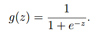
使用sigmoid函数的原因是因为如果用线性拟合的话就会导致预测值可能 >1 or <0，而sigmoid函数恒在这个区间内

from math import e
# 引入自然对数

def Sigmoid(z):
	bottom = 1 + pow(e,-z)
	return 1/bottom
	#我这里的写法可能和后面regularization的时候不大一样，因为不是一天写的代码~

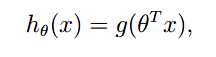
def Hypothesis(x,theta):
	return Sigmoid(theta.T*x)

1.2.2 Cost function and gradient

	代价函数和梯度这里的写法和之前有所区分哦~
	看似梯度和线性回归的式子类似，但是其中的h(x)是不同的

同样来回顾一下logistic回归的代价函数：

梯度：

如果实现顺利的话，我们可以使用theta的初始值带入，获得初始的cost为0.693.

def cost(theta, X, y):
    theta = np.matrix(theta)
    X = np.matrix(X)
    y = np.matrix(y)
    
    first = np.multiply(-y, np.log(hypo(X,theta)))
    # np 的log可以对向量求对数
    second = np.multiply((1 - y), np.log(1 - hypo(X,theta)))
    return np.sum(first - second) / (len(X))

def gradient(theta,X,y):
	# 实现梯度计算，用于库logistics使用的的
	X=np.matrix(X)
	y=np.matrix(y)
	theta=np.matrix(theta)

	parameters = int(theta.ravel().shape[1])
	grad = np.zeros(parameters)

	error=hypo(X,theta)-y
	for i in range(parameters):
		term = np.multiply(error,X[:,i])
		grad[i]=np.sum(term)/len(X)

	return grad

数据预处理部分省略，和线性回归类似
进行测试：

print(cost(theta,X,y))

输出：

 0.6931471805599453

1.2.3 Learning parameters using fminunc

	高级优化算法，这里的算法是matlab里面的。（下面一段话是引用的）

这次，我们不自己写代码实现梯度下降，我们会调用一个已有的库。这就是说，我们不用自己定义迭代次数和步长，功能会直接告诉我们最优解。
andrew ng在课程中用的是Octave的“fminunc”函数，由于我们使用Python，我们可以用scipy.optimize.fmin_tnc做同样的事情。
（另外，如果对fminunc有疑问的，可以参考下面这篇百度文库的内容https://wenku.baidu.com/view/2f6ce65d0b1c59eef8c7b47a.html ）
如果一切顺利的话，最有θ对应的代价应该是0.203

* scipy的一些内容介绍

我们来看一下python的scipy.optimiza.fmin_tnc吧~
这里如果因为直接安装anaconda，使用anaconda中集成的scipy包报错的问题可以看一下我另一篇文章（https://blog.csdn.net/qq_45040216/article/details/119920676）

scipy中的optimize子包中提供了常用的最优化算法函数实现，我们可以直接调用这些函数完成我们的优化问题。

scipy.optimize包提供了几种常用的优化算法。 该模块包含以下几个方面

• 使用各种算法(例如BFGS，Nelder-Mead单纯形，牛顿共轭梯度，COBYLA或SLSQP)的无约束和约束最小化多元标量函数(minimize())
• 全局(蛮力)优化程序(例如，anneal()，basinhopping())
• 最小二乘最小化(leastsq())和曲线拟合(curve_fit())算法
• 标量单变量函数最小化(minim_scalar())和根查找(newton())
• 使用多种算法(例如，Powell，Levenberg-Marquardt混合或Newton-Krylov等大规模方法)的多元方程系统求解

fmin_tnc()

调用：

scipy.optimize.fmin_tnc(func, x0, fprime=None, args=(), approx_grad=0, bounds=None, epsilon=1e-08, scale=None, offset=None, messages=15, maxCGit=-1, maxfun=None, eta=-1, stepmx=0, accuracy=0, fmin=0, ftol=-1, xtol=-1, pgtol=-1, rescale=-1, disp=None, callback=None)

最常使用的参数：

• func：优化的目标函数
• x0：初值
• fprime：提供优化函数func的梯度函数，不然优化函数func必须返回函数值和梯度，或者设置approx_grad=True
• approx_grad :如果设置为True，会给出近似梯度
• args：元组，是传递给优化函数的参数

返回：

• x ： 数组，返回的优化问题目标值
• nfeval ： 整数，function evaluations的数目。
  在进行优化的时候，每当目标优化函数被调用一次，就算一个function evaluation。在一次迭代过程中会有多次function evaluation。这个参数不等同于迭代次数，而往往大于迭代次数。
• rc ： int,Return code, see below

使用scipy

接下来使用：

result = opt.fmin_tnc(func=cost,x0=theta,fprime=gradient,args=(X,y))
print(result)

[out]:

array([-25.16131866,   0.20623159,   0.20147149]), 36, 0

array数组中存放的是最优的theta参数

我们来看一下最优的cost是多少：0.203

# 注意这个result 这个result本身是一个数组，数组的第一项是array数组
# 所以theta0 = result[0][0]
theta_new = np.matrix(result[0])
# 计算这个theta的代价
cost = cost(theta_new,X,y)
print(cost)

[out]:

0.2034977015894744

1.2.4 绘制决策边界

positive = data[data['Admitted'].isin([1])]
negative = data[data['Admitted'].isin([0])]
fig, ax = plt.subplots(figsize=(12, 8))      # 获取绘图对象
# 对录取的数据根据两次考试成绩绘制散点图
ax.scatter(positive['Exam 1'], positive['Exam 2'], s=30, c='b', marker='o', label='Admitted')
# 对未被录取的数据根据两次考试成绩绘制散点图
ax.scatter(negative['Exam 1'], negative['Exam 2'], s=30, c='r', marker='x', label='Not Admitted')

ax.legend()
ax.set_xlabel('Exam 1 Score')
ax.set_ylabel('Exam 2 Score')

x_prex = np.linspace(30,100,100)
y_prex = (-result[0][0]-result[0][1]*x_prex)/result[0][2]
ax.plot(x_prex,y_prex,'y',label='prediction')
# 此处的y是指黄色曲线
ax.legend()
# plt.show()

图如下：

1.2.5 Evaluating logistic regression

	对一个学生预测其录取概率：第一次考试成绩：45；第二次考试成绩：85

首先先定义一个预测函数

# 定义预测函数
def predict_fun(theta,X):
	probability = hypo(X,theta)
	return [1 if x>=0.5 else 0 for x in probability]
	# 返回一个数组项，如果x>=0.5 则数组项为1

score=[1,45,85]
predict=hypo(score,theta_new)
print(predict)

评估这个模型的准确性：

# 评估准确性
# 通过比对训练集
X=np.matrix(X)
predictions = predict_fun(theta_new,X)
# correct = [1 if ((a == 1 and b == 1) or (a == 0 and b == 0)) else 0 for (a, b) in zip(predictions, y)]
# accuracy = (sum(map(int, correct)) % len(correct))
# print ('accuracy = {0}%'.format(accuracy))
correct=0
y=np.matrix(y)
for i in range(len(y)):
	if predictions[i] == y[i]:
		correct+=1
print('accuracy = '+str(correct)+ '%')

1.3 完整代码

# 只需要提供 cost函数和 计算梯度的函数
# python中可以使用scipy.optimize.fmin_tnc做同样的事情

import numpy as np
import pandas as pd
import matplotlib.pyplot as plt
import scipy.optimize as opt

from math import e

def Sigmoid(z):
	bottom = 1 + np.exp(-z)
	return 1/bottom

def hypo(X,theta):
	return Sigmoid(X*theta.T)
	# 此处根据报错修改为X在前

def cost(theta, X, y):
    theta = np.matrix(theta)
    X = np.matrix(X)
    y = np.matrix(y)
    first = np.multiply(-y, np.log(hypo(X,theta)))
    second = np.multiply((1 - y), np.log(1 - hypo(X,theta)))
    return np.sum(first - second) / (len(X))

def gradient(theta,X,y):
	# 实现梯度计算，用于库logistics使用的的
	X=np.matrix(X)
	y=np.matrix(y)
	theta=np.matrix(theta)

	parameters = int(theta.ravel().shape[1])
	grad = np.zeros(parameters)

	error=hypo(X,theta)-y
	for i in range(parameters):
		term = np.multiply(error,X[:,i])
		grad[i]=np.sum(term)/len(X)

	return grad

# 定义预测函数
def predict_fun(theta,X):
	probability = hypo(X,theta)
	return [1 if x>=0.5 else 0 for x in probability]


path = 'ex2data1.txt'
data = pd.read_csv(path,header=None,names=['Exam 1','Exam 2','Admitted'])

data.insert(0,'Ones',1)

cols = data.shape[1]
X=data.iloc[:,0:cols-1]
y=data.iloc[:,cols-1:cols]
theta=np.zeros(3)
print(X.shape,y.shape,theta.shape)

result = opt.fmin_tnc(func=cost,x0=theta,fprime=gradient,args=(X,y))
print(result)
# (array([-25.16131866,   0.20623159,   0.20147149]), 36, 0)
# 此处输出的是theta参数矩阵

theta_new = np.matrix(result[0])
# 计算这个theta的代价
cost = cost(theta_new,X,y)
print(cost)
# 0.2034977015894744

# 画出曲线
positive = data[data['Admitted'].isin([1])]
negative = data[data['Admitted'].isin([0])]
fig, ax = plt.subplots(figsize=(12, 8))      # 获取绘图对象
# 对录取的数据根据两次考试成绩绘制散点图
ax.scatter(positive['Exam 1'], positive['Exam 2'], s=30, c='b', marker='o', label='Admitted')
# 对未被录取的数据根据两次考试成绩绘制散点图
ax.scatter(negative['Exam 1'], negative['Exam 2'], s=30, c='r', marker='x', label='Not Admitted')

ax.legend()
ax.set_xlabel('Exam 1 Score')
ax.set_ylabel('Exam 2 Score')

x_prex = np.linspace(30,100,100)
y_prex = (-result[0][0]-result[0][1]*x_prex)/result[0][2]
ax.plot(x_prex,y_prex,'y',label='prediction')
# 此处的y是指黄色曲线
ax.legend()
# plt.show()

score=[1,45,85]
predict=hypo(score,theta_new)
print(predict)
# 为什么此处精度不如别人？

# 评估准确性
# 通过比对训练集
X=np.matrix(X)
predictions = predict_fun(theta_new,X)
# correct = [1 if ((a == 1 and b == 1) or (a == 0 and b == 0)) else 0 for (a, b) in zip(predictions, y)]
# accuracy = (sum(map(int, correct)) % len(correct))
# print ('accuracy = {0}%'.format(accuracy))
correct=0
y=np.matrix(y)
for i in range(len(y)):
	if predictions[i] == y[i]:
		correct+=1
print('accuracy = '+str(correct)+ '%')

2 Regularized logistic regression

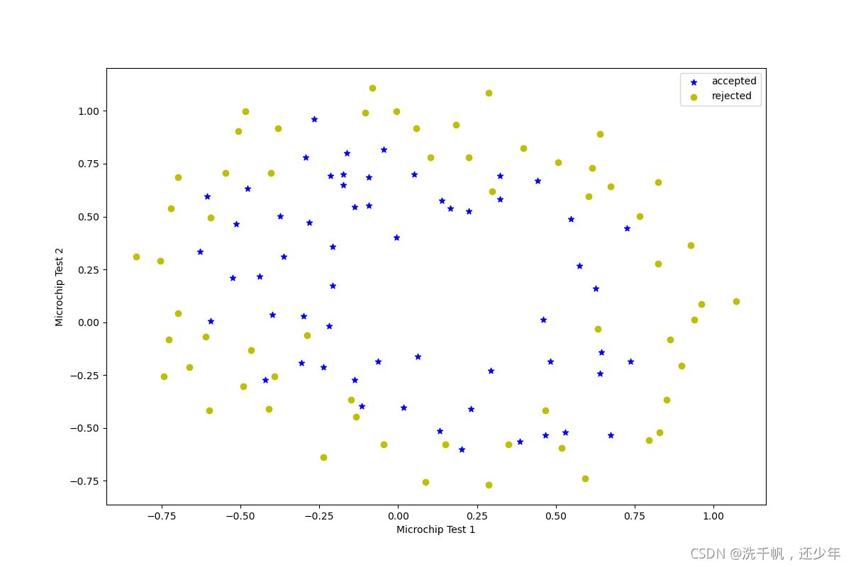
	设想你是工厂的生产主管，你有一些芯片在两次测试中的测试结果，测试结果决定是否芯片要被接受或丢弃。你有一些历史数据，帮助你构建一个逻辑回归模型。

2.1 Visualizing the data

这边就不在赘述了，直接上图和代码

import numpy as np
import pandas as pd
import matplotlib.pyplot as plt

path = 'ex2data2.txt'
data = pd.read_csv(path,header=None,names=['Test 1','Test 2','Result'])

positive = data[data['Result'].isin([1])]
negative = data[data['Result'].isin([0])]

fig,ax=plt.subplots(figsize=(12,8))
ax.scatter(positive['Test 1'],positive['Test 2'],c='b',marker='*',label='accepted')
ax.scatter(negative['Test 1'],negative['Test 2'],c='y',marker='o',label='rejected')
ax.legend()
ax.set_xlabel('Microchip Test 1')
ax.set_ylabel('Microchip Test 2')
plt.show()

2.2 Feature mapping

我们可以看到这个数据用直线显然是无法拟合的。而原有的逻辑回归只适用于线性的分割，所以，这个数据集不适合直接使用逻辑回归。
所以我们可以使用特征映射的方式，增加多项式项。

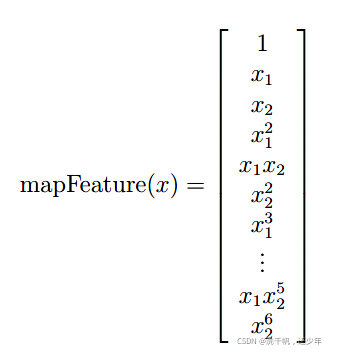
将特征增加到6维，这里使用一个循环

degree = 6
path = 'ex2data2.txt'
data = pd.read_csv(path,names=['Test 1','Test 2','accepted'])
positive = data[data['accepted'].isin([1])]
negative = data[data['accepted'].isin([0])]

x1 = data['Test 1']
x2 = data['Test 2']
# 根据之后的循环及删除操作，1在第三列可以保持最终在第一列
data.insert(3,'Ones',1)

for i in range(1, degree+1):
	# 从1次到6次
    for j in range(0, i+1):
        data['F' + str(i-j) + str(j)] = np.power(x1, i-j) * np.power(x2, j)
        # 直接用x1、x2的次数作为标记，即从F10开始（同时作为列的名称）

# 此处是为了删除前两列
# data.drop('Test 1', axis=1, inplace=True)
# # axis修改即对列进行操作
# data.drop('Test 2', axis=1, inplace=True)

data.drop(['Test 1','Test 2'],axis=1,inplace=True)
print(data.shape)

修改完的数据如下：

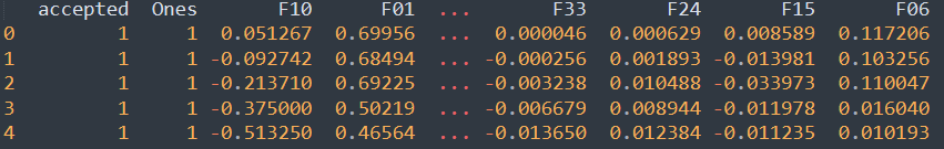
但是我们知道**，增加维度可以增加拟合程度，但同样可能造成过拟合**，这就是为什么我们提出了正则化（regularization）
利用正则化可以很好地避免过拟合的问题，但是如果正则参数设置的不合适，会导致欠拟合（bias 过大）

2.3 Cost function and gradient

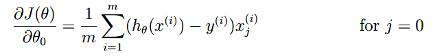
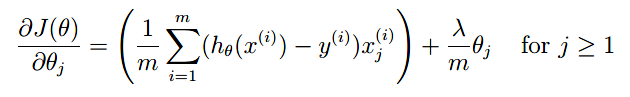
来先回忆一下 正则逻辑回归的 cost function 和梯度，再进行实现：

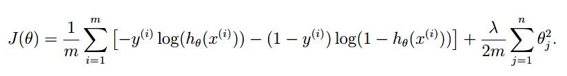
注意梯度：我们只对j不等于0的项进行惩罚

def sigmoid(z):
	return 1/(1 + np.exp(-z))

# 代价函数
def cost(theta,X,y,learningRate):
# 注意形参！
	theta=np.matrix(theta)
	X=np.matrix(X)
	y=np.matrix(y)

	m = len(X)
	first = np.multiply(-y,np.log(sigmoid(X*theta.T)))
	second = np.multiply((1-y),np.log(1-sigmoid(X*theta.T)))
	punish = (learningRate/(2*len(X))) * np.sum(np.power(theta[:,1:theta.shape[1]],2))
	# 此处要将所有theta都进行处理
	return np.sum(first-second)/m + punish

# 梯度
def gradient(theta,X,y,learningRate):
	theta=np.matrix(theta)
	X=np.matrix(X)
	y=np.matrix(y)

	parameters = int(theta.ravel().shape[1])
	grad = np.zeros(parameters)

	error = sigmoid(X*theta.T) - y

	for i in range(parameters):
		term = np.multiply(error,X[:,i])
		# X[:,i] 就是取所有行的第i列的元素。
		if (i == 0):
			grad[i] = np.sum(term)/len(X)
			# 0项不需要加惩罚项
		else:
			grad[i] = (np.sum(term) / len(X)) + ((learningRate / len(X)) * theta[:,i])

	return grad

2.3.1 Learning parameters using fminunc

和上篇类似~
但是注意：
cost、gradient函数 需要第一个形参为theta！！！

cols = data.shape[1]
X=data.iloc[:,1:cols]
y=data.iloc[:,0:1]
# 第一列是接受与不接受

theta =np.matrix(np.zeros(cols-1)) 
# (1,28)

X=np.array(X.values)
# (118,28)
y=np.array(y.values)
learningRate = 1

cost_demo=cost(theta,X,y,learningRate)
print(cost_demo)
# 0.6931471805599454

result = opt.fmin_tnc(func=cost,x0=theta,fprime=gradient,args=(X,y,learningRate))
print(result)

2.3.2 准确率

我们用上一个part的预测函数。
评估一下这个模型的准确率：

# 准确率
# 定义预测函数
def predict(theta,X):
	probability = sigmoid(X*theta.T)
	return [1 if x>=0.5 else 0 for x in probability]

theta_min = np.matrix(result[0])
predictions = predict(theta_min, X)
correct = [1 if ((a == 1 and b == 1) or (a == 0 and b == 0)) else 0 for (a, b) in zip(predictions, y)]
accuracy = (sum(map(int, correct)) % len(correct))
print ('accuracy = {0}%'.format(accuracy))

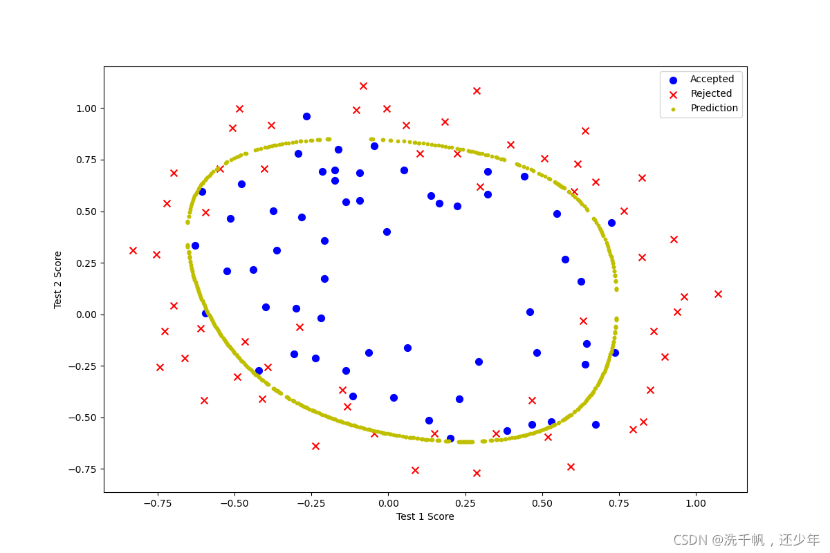
2.4 Plotting the decision boundary

这边的绘图是将决策边界分为左右两部分完成的

def hfunc2(theta, x1, x2):
    temp = theta[0][0]
    place = 0
    for i in range(1, degree+1):
        for j in range(0, i+1):
            temp+= np.power(x1, i-j) * np.power(x2, j) * theta[0][place+1]
            place+=1
    return temp


def find_decision_boundary(theta):
    t1 = np.linspace(-1, 1.5, 1000)
    t2 = np.linspace(-1, 1.5, 1000)

    cordinates = [(x, y) for x in t1 for y in t2]
    x_cord, y_cord = zip(*cordinates)
    h_val = pd.DataFrame({'x1':x_cord, 'x2':y_cord})
    h_val['hval'] = hfunc2(theta, h_val['x1'], h_val['x2'])

    decision = h_val[np.abs(h_val['hval']) < 2 * 10**-3]
    return decision.x1, decision.x2

引用部分：

fig, ax = plt.subplots(figsize=(12,8))
ax.scatter(positive['Test 1'], positive['Test 2'], s=50, c='b', marker='o', label='Accepted')
ax.scatter(negative['Test 1'], negative['Test 2'], s=50, c='r', marker='x', label='Rejected')
ax.set_xlabel('Test 1 Score')
ax.set_ylabel('Test 2 Score')

x, y = find_decision_boundary(result)
plt.scatter(x, y, c='y', s=10, label='Prediction')
ax.legend()
plt.show()

# x = np.linspace(-1, 1.5, 250)
# xx, yy = np.meshgrid(x, x)  #生成网格点坐标矩阵 https://blog.csdn.net/lllxxq141592654/article/details/81532855
# z = feature_mapping(xx.ravel(), yy.ravel(), 6)  #xx,yy都是（250，250）矩阵，经过ravel后，全是(62500,1)矩阵。之后进行特征变换获取(62500,28)的矩阵
# z = z @ theta_res   #将每一行多项式与系数θ相乘，获取每一行的值=θ_0+θ_1*X_1+...+θ_n*X_n
# z = np.array([z]).reshape(xx.shape) #将最终值转成250行和250列坐标
# print(z)
# plt.contour(xx, yy, z, 0)   #传入的xx,yy需要同zz相同维度。
#                             # 其实xx每一行都是相同的，yy每一列都是相同的，所以本质上来说xx是决定了横坐标，yy决定了纵坐标.
#                             # 而z中的每一个坐标都是对于(x,y)的值---即轮廓高度。
#                             # 第四个参数如果是int值，则是设置等高线条数为n+1---会自动选取最全面的等高线。　　如何选取等高线？具体原理还要考虑：是因为从所有数据中找到数据一样的点？
#                             # https://blog.csdn.net/lanchunhui/article/details/70495353
#                             # https://matplotlib.org/api/_as_gen/matplotlib.pyplot.contour.html#matplotlib.pyplot.contour
# plt.show()

2.5 完整代码

import numpy as np
import pandas as pd
import math
import scipy.optimize as opt
import matplotlib.pyplot as plt

def sigmoid(z):
	return 1/(1 + np.exp(-z))

# 代价函数
def cost(theta,X,y,learningRate):
	theta=np.matrix(theta)
	X=np.matrix(X)
	y=np.matrix(y)

	m = len(X)
	first = np.multiply(-y,np.log(sigmoid(X*theta.T)))
	second = np.multiply((1-y),np.log(1-sigmoid(X*theta.T)))
	punish = (learningRate/(2*len(X))) * np.sum(np.power(theta[:,1:theta.shape[1]],2))
	# 此处要将所有theta都进行处理
	return np.sum(first-second)/m + punish

# 梯度
def gradient(theta,X,y,learningRate):
	theta=np.matrix(theta)
	X=np.matrix(X)
	y=np.matrix(y)

	parameters = int(theta.ravel().shape[1])
	grad = np.zeros(parameters)

	error = sigmoid(X*theta.T) - y

	for i in range(parameters):
		term = np.multiply(error,X[:,i])
		# X[:,i] 就是取所有行的第i列的元素。
		if (i == 0):
			grad[i] = np.sum(term)/len(X)
		else:
			grad[i] = (np.sum(term) / len(X)) + ((learningRate / len(X)) * theta[:,i])

	return grad

# 数据预处理
degree = 6
path = 'ex2data2.txt'
data = pd.read_csv(path,names=['Test 1','Test 2','accepted'])
positive = data[data['accepted'].isin([1])]
negative = data[data['accepted'].isin([0])]

x1 = data['Test 1']
x2 = data['Test 2']
data.insert(3,'Ones',1)

for i in range(1, degree+1):
	# 从1次到6次
    for j in range(0, i+1):
        data['F' + str(i-j) + str(j)] = np.power(x1, i-j) * np.power(x2, j)
        # 直接用x1、x2的次数作为标记，即从F10开始（同时作为列的名称）

data.drop(['Test 1','Test 2'],axis=1,inplace=True)

# 设置X，y
cols = data.shape[1]
X=data.iloc[:,1:cols]
y=data.iloc[:,0:1]

theta =np.matrix(np.zeros(cols-1)) 
# (1,28)

X=np.array(X.values)
# (118,28)
y=np.array(y.values)
learningRate = 1

cost_demo=cost(theta,X,y,learningRate)
print(cost_demo)
# 0.6931471805599454

result = opt.fmin_tnc(func=cost,x0=theta,fprime=gradient,args=(X,y,learningRate))
print(result)

def predict(theta,X):
	probability = sigmoid(X*theta.T)
	return [1 if x>=0.5 else 0 for x in probability]

theta_min = np.matrix(result[0])
predictions = predict(theta_min, X)
correct = [1 if ((a == 1 and b == 1) or (a == 0 and b == 0)) else 0 for (a, b) in zip(predictions, y)]
accuracy = (sum(map(int, correct)) % len(correct))
print ('accuracy = {0}%'.format(accuracy))


def hfunc2(theta, x1, x2):
    temp = theta[0][0]
    place = 0
    for i in range(1, degree+1):
        for j in range(0, i+1):
            temp+= np.power(x1, i-j) * np.power(x2, j) * theta[0][place+1]
            place+=1
    return temp


def find_decision_boundary(theta):
    t1 = np.linspace(-1, 1.5, 1000)
    t2 = np.linspace(-1, 1.5, 1000)

    cordinates = [(x, y) for x in t1 for y in t2]
    x_cord, y_cord = zip(*cordinates)
    h_val = pd.DataFrame({'x1':x_cord, 'x2':y_cord})
    h_val['hval'] = hfunc2(theta, h_val['x1'], h_val['x2'])

    decision = h_val[np.abs(h_val['hval']) < 2 * 10**-3]
    return decision.x1, decision.x2

fig, ax = plt.subplots(figsize=(12,8))
ax.scatter(positive['Test 1'], positive['Test 2'], s=50, c='b', marker='o', label='Accepted')
ax.scatter(negative['Test 1'], negative['Test 2'], s=50, c='r', marker='x', label='Rejected')
ax.set_xlabel('Test 1 Score')
ax.set_ylabel('Test 2 Score')

x, y = find_decision_boundary(result)
plt.scatter(x, y, c='y', s=10, label='Prediction')
ax.legend()
plt.show()