


任务一代码
import pandas as pd
import numpy as np
import matplotlib.pyplot as plt
import scipy.optimize as opt
#数据导入
path =r'D:\旧盘\研究生部分\吴恩达 机器学习\ex2-logistic regression\ex2data1.txt'
data = pd.read_csv(path,header=None,names=['test1','test2','result'])
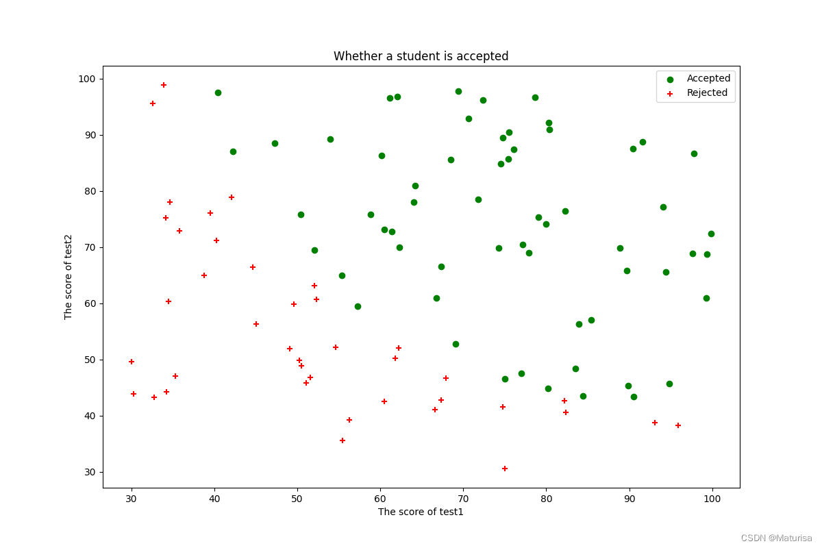
#数据图像化
fig,ax = plt.subplots(figsize=(12,8))
pos_data = data[data.result==1]
neg_data = data[data.result==0]
ax.scatter(pos_data.test1,pos_data.test2,c='g',marker='o',label='Accepted')
ax.scatter(neg_data.test1,neg_data.test2,c='r',marker='+',label='Rejected')
ax.legend(loc=1)
ax.set_xlabel('The score of test1')
ax.set_ylabel('The score of test2')
ax.set_title('Whether a student is accepted')
plt.show()
#数据处理
data.insert(0,'ones',1)
cols = data.shape[1]
x = data.iloc[:,:cols-1]
y = data.iloc[:,cols-1:]
X = np.matrix(x.values)
y = np.matrix(y.values)
theta = np.matrix([0,0,0])
print(X.shape,y.shape,theta.shape)
#激活函数
def sigmoid(z):
return 1/(1+np.exp(-z))
#代价函数
def cost(theta,X,y):
theta = np.matrix(theta)
X = np.matrix(X)
y = np.matrix(y)
left = np.multiply(-y, np.log(sigmoid(X @ theta.T)))
right = np.multiply((1 - y), np.log(1 - sigmoid(X @ theta.T)))
return np.sum(left - right) / (len(X))
print('original cost:',cost(theta,X,y))
#梯度下降
def gradient(theta, X, y):
theta = np.matrix(theta)
X = np.matrix(X)
y = np.matrix(y)
para = theta.shape[1]
grad = np.matrix(np.zeros(para))
error = sigmoid(X @ theta.T) - y
for i in range(3):
grad[0,i] = np.sum(np.multiply(X[:, i], error)) / len(X)
return grad
def predict(theta, X):
theta = np.matrix(theta)
temp = sigmoid(X * theta.T)
print('temp:',temp)
return [1 if x >= 0.5 else 0 for x in temp]
#求theta
result = opt.fmin_tnc(func=cost,x0=theta,fprime = gradient,args=(X,y))
print('result:',result)
Theta = result[0]
print('Theta:',Theta)
#算准确度
predictValues=predict(Theta,X)
hypothesis=[1 if a==b else 0 for (a,b)in zip(predictValues,y)]
accuracy=hypothesis.count(1)/len(hypothesis)
print ('accuracy = {0}%'.format(accuracy*100))
#估计数值
predict1 = 1*Theta[0] + 77*Theta[1] + 47*Theta[2]
print('predict1:',predict1)
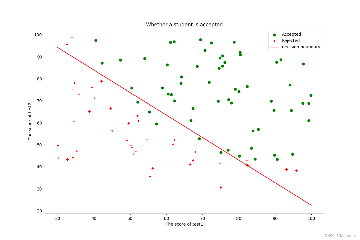
#决策边界
def find_x2(x1,Theta):
return [(-Theta[0]-Theta[1]*x_1)/Theta[2] for x_1 in x1]
x1 = np.linspace(30, 100, 1000)
x2=find_x2(x1,Theta)
#数据可视化
fig,ax = plt.subplots(figsize=(12,8))
pos_data = data[data.result==1]
neg_data = data[data.result==0]
ax.scatter(pos_data.test1,pos_data.test2,c='g',marker='o',label='Accepted')
ax.scatter(neg_data.test1,neg_data.test2,c='r',marker='+',label='Rejected')
ax.plot(x1,x2,color='r',label="decision boundary")
ax.legend(loc=1)
ax.set_xlabel('The score of test1')
ax.set_ylabel('The score of test2')
ax.set_title('Whether a student is accepted')
plt.show()
original cost: 0.6931471805599453
accuracy = 89.0%
Theta: [-25.16131865 0.20623159 0.20147149]
=========================================================================
任务二代码
import pandas as pd
import numpy as np
import matplotlib.pyplot as plt
import warnings
warnings.simplefilter(action='ignore', category=FutureWarning) #关闭熊猫警告,忽略就行
import scipy.optimize as opt
'''函数定义部分'''
# 创建多项式特征变量
def feature(x1,x2,degree):
for i in range(1,degree+1):
for j in range(0,i+1):
data['x1^'+str(i-j),'*x2^'+str(j)]=np.power(x1,i-j)*np.power(x2,j)
return data
#多项式特征变量对应的函数值
def feature_cal(x1,x2,degree,Theta):
res=0
deg=0
for i in range(degree+1):
for j in range(i+1):
res+=x1**j*x2**(i-j)*Theta[0,deg]
deg+=1
return res #res即Theta下y的值
#激活函数
def sigmoid(z):
return 1/(1+np.exp(-z))
#代价函数(带正则)
def costReg(theta,X,y,learningRate):
X = np.matrix(X)
y = np.matrix(y)
theta = np.matrix(theta)
first = np.multiply(-y, np.log(sigmoid(X @ theta.T)))
second = np.multiply(1 - y, np.log(1 - sigmoid(X @ theta.T)))
reg = (learningRate / (2 * len(X))) * np.sum(np.power(theta[:, 1:], 2))
return np.sum(first - second) / len(X) + reg
#梯度下降(带正则)
def gradient(theta,X,y,lbd):
theta = np.matrix(theta)
X = np.matrix(X)
y = np.matrix(y)
para = theta.shape[1]
grad = np.matrix(np.zeros(para))
error = sigmoid(X @ theta.T) - y
for i in range(int(para)):
grad[0, i] =(lbd * np.sum(np.multiply(X[:, i], error)) )/ len(X) #这个就是代价函数的导数,也是梯度下降的步长
return grad
#精确度
def predict(Theta, X):
# Theta = np.matrix(Theta)
temp = sigmoid(X * Theta.T)
# print('temp:',temp)
return [1 if x >= 0.5 else 0 for x in temp]
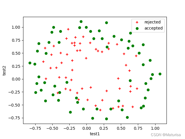
#画散点图
def plot_data(data):
pos_data = data[data.result == 1]
neg_data = data[data.result == 0]
plt.scatter(pos_data.test1, pos_data.test2, c='r', marker='+', label='rejected')
plt.scatter(neg_data.test1, neg_data.test2, c='g', marker='o', label='accepted')
plt.xlabel('test1')
plt.ylabel('test2')
'''开始计算部分'''
#读取数据
path = r'D:\旧盘\研究生部分\吴恩达 机器学习\ex2-logistic regression\ex2data2.txt'
data = pd.read_csv(path,header=None,names=['test1','test2','result'])
print(data.head())
print(data.describe())
#画原始图
plt.figure('raw data')
plot_data(data)
plt.legend(loc=1)
plt.show()
#计算扩展后的特征变量,获得data集
data = feature(data.test1,data.test2,6)
print(type(data.test1))
data.drop("test1",axis=1,inplace=True) #删除列需要axis=1;参数inplace 默认情况下为False,表示保持原来的数据不变,True 则表示在原来的数据上改变。
data.drop("test2",axis=1,inplace=True)
data.insert(1,'Ones',1)
print(data.head())
#用data集创建X,y矩阵
x = data.iloc[:,1:]
y = data.iloc[:,:1]
X = np.matrix(x.values)
y = np.matrix(y.values)
theta = np.matrix(np.zeros(X.shape[1]))
print(X.shape,y.shape,theta.shape)
# print(X,y,theta)
# print(type(x),type(y),type(theta))
#用公式求Theta,调参
lbd = 1
result = opt.fmin_tnc(func=costReg,x0=theta,fprime = gradient,args=(X,y,lbd))
# result = opt.minimize(fun=costReg, args=(X, y, lbd), jac=gradient, x0=theta, method='TNC')
print('result:',result)
print('============================')
Theta = result[0]
Theta = np.matrix(Theta)
print('Theta:',Theta)
print('============================')
print('original cost:',costReg(theta,X,y,learningRate=1))
print('============================')
print('current cost:',costReg(Theta,X,y,learningRate=1))
#算准确度
predict = predict(Theta, X)
# print('predict:',predict)
hypothesis=[1 if a==b else 0 for (a,b)in zip(predict,y)]
accuracy=hypothesis.count(1)/len(hypothesis)
print('============================')
print ('accuracy = {0}%'.format(accuracy*100))
#画拟合函数图
x_axis = np.linspace(-1, 1, 100)
y_axis = np.linspace(-1, 1, 100)
zz = np.zeros((x_axis.size, y_axis.size))
for xs in range(x_axis.size):
for ys in range(y_axis.size):
zz[xs, ys] = feature_cal(x_axis[xs], y_axis[ys], 6, Theta)
data = pd.read_csv(path,header=None,names=['test1','test2','result']) #这里注意必须再写一遍,因为在93行,data已经变成特征变量增多后的数据了。下次注意将原始数据用data_raw来命名。
plt.figure('decision_boundary')
plot_data(data)
plt.contour(x_axis,y_axis,zz,0,colors='y',label='boundary') #函数值为0代表决策边界
plt.legend(loc=1)
plt.show()
original cost: 0.6931471805599454
accuracy = 84.7457627118644%
Theta: [[ 1.60695456 1.1560186 1.96230284 -3.0506508 -1.65702971 -1.91905201
0.57020964 -0.68153388 -0.71446988 0.04581342 -2.05403849 -0.19543701
-1.06002879 -0.50146813 -1.49394535 0.08870346 -0.37553871 -0.1621286
-0.47670397 -0.49928213 -0.25753424 -1.25322562 0.00804809 -0.51945916
-0.03978315 -0.54273819 -0.21843762 -0.93050987]]


 3938
3938


 被折叠的 条评论
为什么被折叠?
被折叠的 条评论
为什么被折叠?
 到【灌水乐园】发言


