


引言
大家好,我是GISer Liu😁,一名热爱AI技术的GIS开发者。本系列文章是我跟随DataWhale 2024年10月学习赛的Python量化交易学习总结文档。
在现代金融市场中,量化回测是评估投资策略有效性和稳定性的关键步骤。本文将系统梳理量化回测的重要性、基本概念,并详细介绍如何使用Python进行量化回测。
我们将重点解析常见的策略评估指标,如年化收益率、波动率、最大回撤、Alpha系数、Beta系数、夏普比率和信息比率,并通过实际案例展示如何计算这些指标。
此外,本文还将介绍如何在聚宽、Backtrader和BigQuant等平台上实现双均线策略,并进行回测。最后,我们将展示一个本地傻瓜式回测框架,帮助您快速上手量化回测。
通过本文的学习,您将掌握量化回测的核心概念和实用工具,提升在复杂市场环境中的策略评估能力。
一、量化回测框架概述
1. 量化回测的重要性
量化回测是量化投资中不可或缺的一环,通过对历史数据的回测,可以评估策略的有效性和稳定性。本文将详细介绍如何使用Python进行量化回测,并结合实际案例进行讲解。
2. 量化回测的基本概念
- 年化收益率:策略在一年内的预期收益率;该值变大则投资者获得更高回报,反之更低甚至亏损;
- 基准年化收益率:市场基准在一年内的预期收益率。
- 最大回撤:策略在选定周期内可能出现的最大亏损幅度,策略的风险增加,投资者可能面临更大的亏损;
- 波动率:策略收益的波动性,用于衡量风险;波动率越小,收益稳定性越强;
- Alpha系数:策略的超额收益,与市场波动无关,变大则策略收益优于市场收益;
- Beta系数:策略的系统风险,与市场波动相关;较大则对市场波动的敏感性增强。
- 夏普比率:每承受一单位总风险所产生的超额报酬,策略的风险调整后收益增加,表现更优。
- 信息比率:策略相对于基准的超额收益与跟踪误差的比值;该值增大则策略相对于基准的超额收益增加,表现优于基准。
市场上常以年化收益率指标进行股票打分,而实际分数更应该是一个甲醛组合的分数,而非单一指标;
二、使用Python计算策略评估指标
1. 数据准备
在进行量化回测之前,首先需要准备好历史数据。本文将以贵州茅台、工商银行、中国平安为例,使用Tushare获取数据,并计算相关指标。
① 导入必要的库
import pandas as pd
import numpy as np
import matplotlib.pyplot as plt
import tushare as ts
%matplotlib inline

# 无视warning
import warnings
warnings.filterwarnings("ignore")

# 正常显示画图时出现的中文和负号
from pylab import mpl
mpl.rcParams['font.sans-serif']=['SimHei']
mpl.rcParams['axes.unicode_minus']=False
② 获取数据
# 配置 tushare token
my_token = 'XXXXX'
pro = ts.pro_api(my_token)
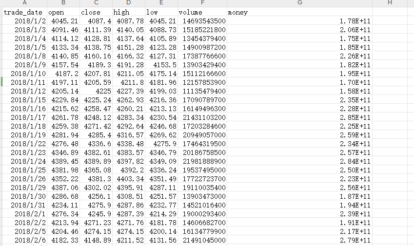
def get_data(code, start_date, end_date):
df = pro.daily(ts_code=code, start_date=start_date, end_date=end_date)
df.index = pd.to_datetime(df.trade_date)
return df.close
# 以上证综指、贵州茅台、工商银行、中国平安为例
stocks={
'600519.SH':'贵州茅台',
'601398.SH':'工商银行',
'601318.SH':'中国平安'
}
df = pd.DataFrame()
for code,name in stocks.items():
df[name] = get_data(code, '20180101', '20221231')
# 按照日期正序
df = df.sort_index()
# 本地读入沪深300合并
df_base = pd.read_csv('000300.XSHG_2018_2022.csv')
df_base.index = pd.to_datetime(df_base.trade_date)
df['沪深300'] = df_base['close']
为什么使用沪深300指数作为基准?
- 代表性:沪深300指数由沪深两市中市值大、流动性好的300只股票组成,覆盖A股市场约70%的市值,被广泛认为是反映中国A股市场整体表现的代表性指数。
- 基准比较:在量化策略回测中,通常将策略表现与沪深300指数进行比较,以评估策略的相对表现。
- 风险调整后收益:通过比较策略收益与沪深300指数收益,可以计算Alpha系数、Beta系数、夏普比率和信息比率等风险调整后收益指标,帮助投资者更好地理解策略的风险和收益特征。
- 市场平均值:沪深300指数包含市场上大部分流动性股票,可视为市场平均值。通过比较,可以评估策略是否跑赢市场平均水平。
- 行业分布:沪深300指数行业分布均衡,涵盖多个主要行业,能较好反映市场整体行业表现。通过比较,可以评估策略在不同行业中的表现。
2. 净值曲线
净值曲线是量化回测中常用的可视化工具,用于展示策略在不同时间点的资产价值相对于期初的倍数。
# 以第一交易日2018年1月1日收盘价为基点,计算净值并绘制净值曲线
df_worth = df / df.iloc[0]
df_worth.plot(figsize=(15,6))
plt.title('股价净值走势', fontsize=10)
plt.xticks(pd.date_range('20180101','20221231',freq='Y'),fontsize=10)
plt.show()
结果如下:
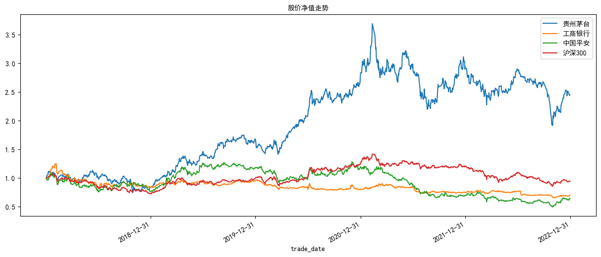
贵州茅台遥遥领先呀!🤣
3. 年化收益率
年化收益率是衡量策略长期表现的重要指标,通过计算策略在一年内的预期收益率,可以评估策略的盈利能力。
① 累计收益率
# 区间累计收益率(绝对收益率)
total_return = df_worth.iloc[-1]-1
total_return = pd.DataFrame(total_return.values,columns=['累计收益率'],index=total_return.index)
print(total_return)
② 年化收益率
# 年化收益率
annual_return = pd.DataFrame((1 + total_return.values) ** (252 / 1826) - 1,columns=['年化收益率'],index=total_return.index)
print(annual_return)
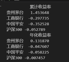
看来只有贵州茅台赚到钱了😂
4. 波动率
波动率(Volatility)是衡量资产价格波动性的指标,通常用于评估投资风险。波动率可以通过多种方法计算,其中最常见的是历史波动率和年化波动率。以下是波动率的计算公式及其详细解释。
- **历史波动率:**是基于资产价格的历史数据计算得出的波动率。它通常使用标准差来衡量价格的变化。
Volatility = 1 n − 1 ∑ i = 1 n ( r i − r ˉ ) 2 \text{Volatility} = \sqrt{\frac{1}{n-1} \sum_{i=1}{n} (r_i - \bar{r})2} Volatility=n−11∑i=1n(ri−rˉ)2
其中:
-
( r i r_i ri) 是第 ( i ) 天的收益率。
-
( r ˉ \bar{r} rˉ) 是收益率的平均值。
-
( n n n) 是收益率的数量。
-
**年化波动率:**是将历史波动率转换为年化形式的波动率。通常假设一年有252个交易日(因为一年中大约有252个交易日)。
Annualized Volatility = Volatility × 252 \text{Annualized Volatility} = \text{Volatility} \times \sqrt{252} Annualized Volatility=Volatility×252
其中:
- ( Volatility \text{Volatility} Volatility) 是历史波动率。
- ( 252 ) 是一年中的交易日数量。
波动率是衡量策略风险的重要指标,通过计算策略收益的标准差,可以评估策略的波动性。
代码如下:
df_return = df / df.shift(1) - 1
df_return = ((df_return.iloc[1:] - df_return.mean()) ** 2)

volatility = pd.DataFrame(np.sqrt(df_return.sum() * 252 / (1826-1)),columns=['波动率'],index=total_return.index)
volatility
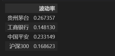
由此看来,工商银行波动最小;
5. 最大回撤
最大回撤计算的是从策略净值的历史最高点(峰值)到随后的最低点(谷值)之间的最大跌幅。它反映了策略在某个时间段内可能面临的最大亏损风险。
最大回撤的计算公式如下:
Max Drawdown = max ( Peak Value − Trough Value Peak Value ) \text{Max Drawdown} = \max \left( \frac{\text{Peak Value} - \text{Trough Value}}{\text{Peak Value}} \right) Max Drawdown=max(Peak ValuePeak Value−Trough Value)
其中:
- Peak Value:策略净值的历史最高点。
- Trough Value:从峰值到谷值之间的最低点。
最大回撤是衡量策略风险的重要指标,通过计算策略在选定周期内可能出现的最大亏损幅度,可以评估策略的抗风险能力。
def max_drawdown_cal(df):
    md = ((df.cummax() - df)/df.cummax()).max()
    return round(md, 4)

max_drawdown = {}

stocks={
    '600519.SH':'贵州茅台',
    '601398.SH':'工商银行',
    '601318.SH':'中国平安',
    '000300.XSHG': '沪深300'
}

for code,name in stocks.items():
    max_drawdown[name]=max_drawdown_cal(df[name])

max_drawdown = pd.DataFrame(max_drawdown,index=['最大回撤']).T
max_drawdown
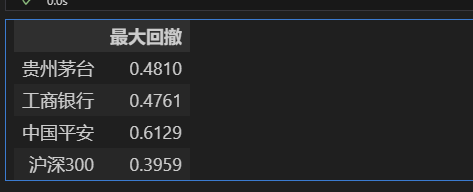
- 最大回撤并不是单日最大亏损,而是衡量策略在选定周期内可能出现的最大亏损幅度的指标;
6. Alpha系数和Beta系数
Alpha系数和Beta系数是资本资产定价模型(CAPM)中的两个重要指标,用于衡量投资组合的风险和收益特征。以下是它们的定义和计算公式。
① Beta系数
Beta系数(β)衡量的是投资组合相对于市场整体(通常是某个基准指数,如沪深300指数)的系统性风险。Beta系数大于1表示投资组合的波动性高于市场,小于1表示波动性低于市场。
公式:
β = Cov ( R p , R m ) Var ( R m ) \beta = \frac{\text{Cov}(R_p, R_m)}{\text{Var}(R_m)} β=Var(Rm)Cov(Rp,Rm)
其中:
- ( R p R_p Rp) 是投资组合的收益率。
- ( R m R_m Rm) 是市场基准的收益率。
- ( Cov ( R p , R m ) \text{Cov}(R_p, R_m) Cov(Rp,Rm)) 是投资组合收益率与市场基准收益率的协方差。
- ( Var ( R m ) \text{Var}(R_m) Var(Rm)) 是市场基准收益率的方差。
② Alpha系数
Alpha系数(α)衡量的是投资组合的超额收益,即投资组合的实际收益率与根据CAPM模型预测的收益率之间的差异。Alpha系数为正表示投资组合的表现优于市场,为负表示表现不如市场。
公式:
α = R p − [ R f + β ( R m − R f ) ] \alpha = R_p - [R_f + \beta (R_m - R_f)] α=Rp−[Rf+β(Rm−Rf)]
其中:
- ( R p R_p Rp) 是投资组合的实际收益率。
- ( R f R_f Rf) 是无风险收益率(通常使用国债收益率)。
- ( β \beta β) 是投资组合的Beta系数。
- ( R m R_m Rm) 是市场基准的收益率。
代码:
# 假设无风险收益率为0.01
R_f = 0.01

# 计算Alpha系数
alpha = R_p.mean() - (R_f + beta * (R_m.mean() - R_f))
print(f"Alpha系数: {alpha}")
- Beta系数:衡量投资组合相对于市场基准的系统性风险,通过协方差和方差计算。
- Alpha系数:衡量投资组合的超额收益,通过实际收益率与CAPM模型预测收益率的差异计算。
对我们的数据进行两个系数的计算;
from scipy import stats

#计算每日收益率 收盘价缺失值(停牌),使用前值代替
rets=(df.iloc[:,:4].fillna(method='pad')).apply(lambda x:x/x.shift(1)-1)[1:]

#市场指数为x,个股收益率为y
x = rets.iloc[:,3].values
y = rets.iloc[:,:3].values
capm = pd.DataFrame()
alpha = []
beta = []
for i in range(3):
    b, a, r_value, p_value, std_err=stats.linregress(x,y[:,i])
    #alpha转化为年化
    alpha.append(round(a*250,3))
    beta.append(round(b,3))

capm['alpha']=alpha
capm['beta']=beta
capm.index=rets.columns[:3]
#输出结果:
capm
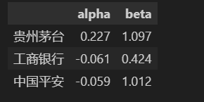
可以看出工商银行最稳定,但是超额收益低于市场平均收益,而贵州茅台超额收益高于市场平均,但是却不够稳定;
7. 夏普比率
夏普比率衡量的是每单位总风险所获得的超额收益。它通过将投资组合的超额收益(即超过无风险利率的收益)除以其标准差来计算。
公式:
Sharpe Ratio = R p − R f σ p \text{Sharpe Ratio} = \frac{R_p - R_f}{\sigma_p} Sharpe Ratio=σpRp−Rf
其中:
- ( R p R_p Rp) 是投资组合的平均收益率。
- ( R f R_f Rf) 是无风险收益率(通常使用国债收益率)。
- ( σ p \sigma_p σp) 是投资组合收益率的标准差。
示例代码:
import numpy as np

# 假设有一组投资组合的收益率数据
R_p = np.array([0.01, -0.02, 0.03, -0.01, 0.02])
R_f = 0.01  # 无风险收益率

# 计算夏普比率
sharpe_ratio = (R_p.mean() - R_f) / R_p.std(ddof=1)
print(f"夏普比率: {sharpe_ratio}")
- NN 是数据点的数量。
- ddof=0:分母为 NN,计算的是总体标准差。
- ddof=1:分母为 N−1N−1,计算的是样本标准差。
- 夏普比率:衡量每单位总风险所获得的超额收益,通过投资组合的超额收益除以其标准差计算。
我们来计算一下之前数据的夏普比率:
# 超额收益率以无风险收益率为基准 假设无风险收益率为年化3%
ex_return=rets - 0.03/250

# 计算夏普比率
sharpe_ratio=np.sqrt(len(ex_return))*ex_return.mean()/ex_return.std()
sharpe_ratio=pd.DataFrame(sharpe_ratio,columns=['夏普比率'])
sharpe_ratio
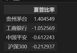
可以看出,贵州茅台具有最高的超额收益,工商银行、中国平安和沪深300还不如买债券;
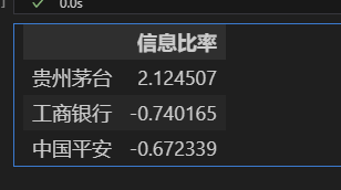
8. 信息比率
信息比率衡量的是投资组合相对于基准的超额收益与跟踪误差的比值。它通过将投资组合的超额收益除以其跟踪误差来计算。
公式:
Information Ratio = R p − R b σ t \text{Information Ratio} = \frac{R_p - R_b}{\sigma_t} Information Ratio=σtRp−Rb
其中:
- ( R p R_p Rp) 是投资组合的平均收益率。
- ( R b R_b Rb) 是基准的平均收益率。
- ( σ t \sigma_t σt) 是投资组合与基准收益率之间的跟踪误差(即超额收益的标准差)。
示例:
# 假设有一组基准的收益率数据
R_b = np.array([0.02, -0.01, 0.04, -0.02, 0.03])

# 计算信息比率
excess_returns = R_p - R_b
information_ratio = excess_returns.mean() / excess_returns.std(ddof=1)
print(f"信息比率: {information_ratio}")
这里我们计算一下上面代码中的信息比率;
#信息比率
ex_return = pd.DataFrame()
ex_return['贵州茅台']=rets.iloc[:,0]-rets.iloc[:,3]
ex_return['工商银行']=rets.iloc[:,1]-rets.iloc[:,3]
ex_return['中国平安']=rets.iloc[:,2]-rets.iloc[:,3]

#计算信息比率
information_ratio = np.sqrt(len(ex_return))*ex_return.mean()/ex_return.std()
#信息比率的输出结果
information_ratio = pd.DataFrame(information_ratio,columns=['信息比率'])
information_ratio
- 信息比率:衡量投资组合相对于基准的超额收益与跟踪误差的比值,通过投资组合的超额收益除以其跟踪误差计算。
三、平台量化回测实践
1.聚宽平台
聚宽(JoinQuant)是一个功能强大的量化交易平台,提供了丰富的数据和工具,帮助用户进行量化策略的开发和回测。
本部分将介绍如何在聚宽平台实现一个双均线策略,并在平台上进行回测,来测试整体收益率。代码如下:
# 导入函数库
from jqdata import *

# 初始化函数,设定基准等等
def initialize(context):
    # 设定沪深上证作为基准
    set_benchmark('000300.XSHG')
    # 开启动态复权模式(真实价格)
    set_option('use_real_price', True)
    # 输出内容到日志 log.info()
    log.info('初始函数开始运行且全局只运行一次')
    # 过滤掉order系列API产生的比error级别低的log
    # log.set_level('order', 'error')

    ### 股票相关设定 ###
    # 股票类每笔交易时的手续费是:买入时佣金万分之三,卖出时佣金万分之三加千分之一印花税, 每笔交易佣金最低扣5块钱
    set_order_cost(OrderCost(close_tax=0.001, open_commission=0.0003, close_commission=0.0003, min_commission=5), type='stock')

    ## 运行函数(reference_security为运行时间的参考标的;传入的标的只做种类区分,因此传入'000300.XSHG'或'510300.XSHG'是一样的)
      # 开盘前运行
    run_daily(before_market_open, time='before_open', reference_security='000300.XSHG')
      # 开盘时运行
    run_daily(market_open, time='open', reference_security='000300.XSHG')
      # 收盘后运行
    run_daily(after_market_close, time='after_close', reference_security='000300.XSHG')

## 开盘前运行函数
def before_market_open(context):
    # 输出运行时间
    log.info('函数运行时间(before_market_open):'+str(context.current_dt.time()))

    # 给微信发送消息(添加模拟交易,并绑定微信生效)
    # send_message('美好的一天~')

    # 要操作的股票:比亚迪(g.为全局变量)
    g.security = '002594.XSHE'

## 开盘时运行函数
def market_open(context):
    log.info('函数运行时间(market_open):'+str(context.current_dt.time()))
    security = g.security
    # 获取股票的收盘价
    close_data5 = get_bars(security, count=5, unit='1d', fields=['close'])
    close_data10 = get_bars(security, count=10, unit='1d', fields=['close'])
    # close_data20 = get_bars(security, count=20, unit='1d', fields=['close'])
    # 取得过去五天,十天的平均价格
    MA5 = close_data5['close'].mean()
    MA10 = close_data10['close'].mean()
    # 取得上一时间点价格
    #current_price = close_data['close'][-1]
    # 取得当前的现金
    cash = context.portfolio.available_cash

    # 五日均线上穿十日均线
    if (MA5 > MA10) and (cash > 0):
        # 记录这次买入
        log.info("5日线金叉10日线,买入 %s" % (security))
        # 用所有 cash 买入股票
        order_value(security, cash)
    # 五日均线跌破十日均线
    elif (MA5 < MA10) and context.portfolio.positions[security].closeable_amount > 0:
        # 记录这次卖出
        log.info("5日线死叉10日线, 卖出 %s" % (security))
        # 卖出所有股票,使这只股票的最终持有量为0
        for security in context.portfolio.positions.keys():
            order_target(security, 0)

## 收盘后运行函数
def after_market_close(context):
    log.info(str('函数运行时间(after_market_close):'+str(context.current_dt.time())))
    #得到当天所有成交记录
    trades = get_trades()
    for _trade in trades.values():
        log.info('成交记录:'+str(_trade))
    log.info('一天结束')
    log.info('##############################################################')
2.Backtrader平台
Backtrader是一款基于Python的开源量化回测框架,功能完善,安装简单,适合量化策略的开发和回测。
本部分将介绍如何在Backtrader实现一个双均线策略,并在平台上进行回测,来测试整体收益率。代码如下:
# 导入函数库
from __future__ import (absolute_import, division, print_function, unicode_literals)
import datetime
import pymysql
import pandas as pd
import backtrader as bt
import tushare as ts
import numpy as np

# 数据获取(从Tushare中获取数据)
def get_data(stock_code):
    """
    stock_code:股票代码,类型: str
    return: 股票日线数据,类型: DataFrame
    """
    token = 'Tushare token'   # 可通过进入个人主页-接口TOKEN获得

    ts.set_token(token)
    pro = ts.pro_api(token)

    data_daily = pro.daily(ts_code = stock_code, start_date='20180101', end_date='20230101')
    data_daily['trade_date'] = pd.to_datetime(data_daily['trade_date'])
    data_daily = data_daily.rename(columns={'vol': 'volume'})
    data_daily.set_index('trade_date', inplace=True)
    data_daily = data_daily.sort_index(ascending=True)
    dataframe = data_daily
    data_daily['openinterest'] = 0
    dataframe['openinterest'] = 0
    data = bt.feeds.PandasData(dataname=dataframe,
                               fromdate=datetime.datetime(2018, 1, 1),
                               todate=datetime.datetime(2023, 1, 1)
                               )

    return data

# 双均线策略实现
class DoubleAverages(bt.Strategy):

    # 设置均线周期
    params = (
        ('period_data5', 5),
        ('period_data10', 10)
    )

    # 日志输出
    def log(self, txt, dt=None):
        dt = dt or self.datas[0].datetime.date(0)
        print('%s, %s' % (dt.isoformat(), txt))

    def __init__(self):
        # 初始化数据参数

        self.dataclose = self.datas[0].close   # 定义变量dataclose,保存收盘价
        self.order = None   # 定义变量order,用于保存订单
        self.buycomm = None    # 定义变量buycomm,记录订单佣金
        self.buyprice = None    # 定义变量buyprice,记录订单价格

        self.sma5 = bt.indicators.SimpleMovingAverage(self.datas[0], period=self.params.period_data5)  # 计算5日均线
        self.sma10 = bt.indicators.SimpleMovingAverage(self.datas[0], period=self.params.period_data10)  # 计算10日均线

    def notify_order(self, order):
        if order.status in [order.Submitted, order.Accepted]:  # 若订单提交或者已经接受则返回
            return

        if order.status in [order.Completed]:
            if order.isbuy():
                self.log(
                    'Buy Executed, Price: %.2f, Cost: %.2f, Comm: %.2f' %
                    (order.executed.price, order.executed.value, order.executed.comm))

                self.buyprice = order.executed.price
                self.buycomm = order.executed.comm
            else:
                self.log('Sell Executed, Price: %.2f, Cost: %.2f, Comm: %.2f' %
                        (order.executed.price, order.executed.value, order.executed.comm))
            self.bar_executed = len(self)
        elif order.status in [order.Canceled, order.Margin, order.Rejected]:
            self.log('Order Canceled/Margin/Rejected')

        self.order = None


    def notify_trade(self, trade):
        if not trade.isclosed:   # 若交易未关闭则返回
            return
        self.log('Operation Profit, Total_Profit %.2f, Net_Profit: %.2f' %
                (trade.pnl, trade.pnlcomm))    # pnl表示盈利, pnlcomm表示手续费

    def next(self):   # 双均线策略逻辑实现
        self.log('Close: %.2f' % self.dataclose[0])   # 打印收盘价格

        if self.order:   # 检查是否有订单发送
            return

        if not self.position:   # 检查是否有仓位
            if self.sma5[0] > self.sma10[0]:
                self.log('Buy: %.2f' % self.dataclose[0])
                self.order = self.buy()

        else:
            if self.sma5[0] < self.sma10[0]:
                self.log('Sell: %.2f' % self.dataclose[0])
                self.order = self.sell()

if __name__ == '__main__':
    cerebro = bt.Cerebro()   # 创建策略容器
    cerebro.addstrategy(DoubleAverages)    # 添加双均线策略
    data = get_data('000001.SZ')
    cerebro.adddata(data)   # 添加数据
    cerebro.broker.setcash(10000.0)   # 设置资金
    cerebro.addsizer(bt.sizers.FixedSize, stake=100)   # 设置每笔交易的股票数量
    cerebro.broker.setcommission(commission=0.01)   # 设置手续费
    print('Starting Portfolio Value: %.2f' % cerebro.broker.getvalue())   # 打印初始资金
    cerebro.run()   # 运行策略
    print('Final Portfolio Value: %.2f' % cerebro.broker.getvalue())   # 打印最终资金
    cerebro.plot()
3.BigQuant量化框架实战
BigQuant是一个人工智能量化投资平台,提供了丰富的数据和工具,帮助用户进行量化策略的开发和回测。
本部分将介绍如何在BigQuant实现一个双均线策略,并在平台上进行回测,来测试整体收益率。代码如下:
from bigdatasource.api import DataSource
from biglearning.api import M
from biglearning.api import tools as T
from biglearning.api import Outputs

import pandas as pd
import numpy as np
import math
import warnings
import datetime

from zipline.finance.commission import PerOrder
from zipline.api import get_open_orders
from zipline.api import symbol

from bigtrader.sdk import *
from bigtrader.utils.my_collections import NumPyDeque
from bigtrader.constant import OrderType
from bigtrader.constant import Direction

def m3_initialize_bigquant_run(context):
    context.set_commission(PerOrder(buy_cost=0.0003, sell_cost=0.0013, min_cost=5))


def m3_handle_data_bigquant_run(context, data):
    today = data.current_dt.strftime('%Y-%m-%d')
    stock_hold_now = {e.symbol: p.amount * p.last_sale_price
                 for e, p in context.perf_tracker.position_tracker.positions.items()}

    cash_for_buy = context.portfolio.cash

    try:
        buy_stock = context.daily_stock_buy[today]
    except:
        buy_stock=[]

    try:
        sell_stock = context.daily_stock_sell[today]
    except:
        sell_stock=[]

    stock_to_sell = [ i for i in stock_hold_now if i in sell_stock ]

    stock_to_buy = [ i for i in buy_stock if i not in stock_hold_now ]

    stock_to_adjust=[ i for i in stock_hold_now if i not in sell_stock ]

    if len(stock_to_sell)>0:
        for instrument in stock_to_sell:
            sid = context.symbol(instrument)
            cur_position = context.portfolio.positions[sid].amount
            if cur_position > 0 and data.can_trade(sid):
                context.order_target_percent(sid, 0)
                cash_for_buy += stock_hold_now[instrument]


    if len(stock_to_buy)+len(stock_to_adjust)>0:
        weight = 1/(len(stock_to_buy)+len(stock_to_adjust))
        for instrument in stock_to_buy+stock_to_adjust:
            sid = context.symbol(instrument)
            if  data.can_trade(sid):
                context.order_target_value(sid, weight*cash_for_buy)

def m3_prepare_bigquant_run(context):
    df = context.options['data'].read_df()

    def open_pos_con(df):
        return list(df[df['buy_condition']>0].instrument)

    def close_pos_con(df):
        return list(df[df['sell_condition']>0].instrument)

    context.daily_stock_buy= df.groupby('date').apply(open_pos_con)

    context.daily_stock_sell= df.groupby('date').apply(close_pos_con)

m1 = M.input_features.v1(
    features="""# #号开始的表示注释
# 多个特征,每行一个,可以包含基础特征和衍生特征
buy_condition=where(mean(close_0,5)>mean(close_0,10),1,0)
sell_condition=where(mean(close_0,5)<mean(close_0,10),1,0)""",
    m_cached=False
)

m2 = M.instruments.v2(
    start_date=T.live_run_param('trading_date', '2019-03-01'),
    end_date=T.live_run_param('trading_date', '2021-06-01'),
    market='CN_STOCK_A',
    instrument_list="""600519.SHA
601392.SHA""",
    max_count=0
)

m7 = M.general_feature_extractor.v7(
    instruments=m2.data,
    features=m1.data,
    start_date='',
    end_date='',
    before_start_days=60
)

m8 = M.derived_feature_extractor.v3(
    input_data=m7.data,
    features=m1.data,
    date_col='date',
    instrument_col='instrument',
    drop_na=False,
    remove_extra_columns=False
)

m4 = M.dropnan.v2(
    input_data=m8.data
)

m3 = M.trade.v4(
    instruments=m2.data,
    options_data=m4.data,
    start_date='',
    end_date='',
    initialize=m3_initialize_bigquant_run,
    handle_data=m3_handle_data_bigquant_run,
    prepare=m3_prepare_bigquant_run,
    volume_limit=0.025,
    order_price_field_buy='open',
    order_price_field_sell='open',
    capital_base=1000000,
    auto_cancel_non_tradable_orders=True,
    data_frequency='daily',
    price_type='后复权',
    product_type='股票',
    plot_charts=True,
    backtest_only=False,
    benchmark='000300.HIX'
)
四、本地傻瓜式回测框架
1. 准备工作
① 安装Talib
conda install -c conda-forge ta-lib
个人推荐这个方法
② 安装hyperopt
pip install hyperopt
③ 准备数据
2. 完整代码
# %% 引入包
import pandas as pd
import math
import matplotlib.pyplot as plt
import talib # http://mrjbq7.github.io/ta-lib/doc_index.html
import numpy as np
from sqlalchemy import create_engine
from hyperopt import tpe, hp, fmin, STATUS_OK, Trials
from hyperopt.pyll.base import scope
import importlib
import warnings
warnings.filterwarnings('ignore')
plt.rcParams['font.sans-serif'] = 'SimHei'
plt.rcParams['axes.unicode_minus'] = False
# %% 自定义函数
def setpos(pos, *args):
HQDf = args[1]
idx = args[2]
HQDf.loc[idx, 'pos'] = pos
def CalculateResult(HQDf):
def get_max_drawdown(array):
array = pd.Series(array)
cummax = array.cummax()
return array / cummax - 1
HQDf = HQDf.fillna(0)
HQDf['base_balance'] = HQDf.close / HQDf.close[0] # 基准净值
HQDf['chg'] = HQDf.close.pct_change() # 单日涨跌幅
# 计算策略净值
HQDf['strategy_balance'] = 1.0
for i in range(0, len(HQDf)):
if i > 0:
HQDf.loc[HQDf.index[i], 'strategy_balance'] = HQDf.iloc[i - 1]['strategy_balance'] * (1. + HQDf.iloc[i]['chg'] * HQDf.iloc[i - 1]['pos'])
HQDf['drawdown'] = get_max_drawdown(HQDf['strategy_balance']) # 回撤
StatDf = {}
StatDf['MaxDrawDown'] = min(HQDf['drawdown']) # 最大回撤
StatDf['return'] = HQDf['strategy_balance'][-1] - 1 # 区间收益
# 计算年化收益
years = (HQDf.index[-1] - HQDf.index[0]).days / 365
if years <= 1:
StatDf['yearReturn'] = StatDf['return'] / years
else:
StatDf['yearReturn'] = (HQDf['strategy_balance'][-1] / 1) ** (1 / years) - 1
StatDf['return/maxdrawdown'] = -1 * StatDf['return'] / StatDf['MaxDrawDown']
# 计算夏普比
x = HQDf["strategy_balance"] / HQDf["strategy_balance"].shift(1)
x[x <= 0] = np.nan
HQDf["return"] = np.log(x).fillna(0)
daily_return = HQDf["return"].mean() * 100
return_std = HQDf["return"].std() * 100
daily_risk_free = 0.015 / np.sqrt(240)
StatDf['sharpe_ratio'] = (daily_return - daily_risk_free) / return_std * np.sqrt(240)
return HQDf, StatDf
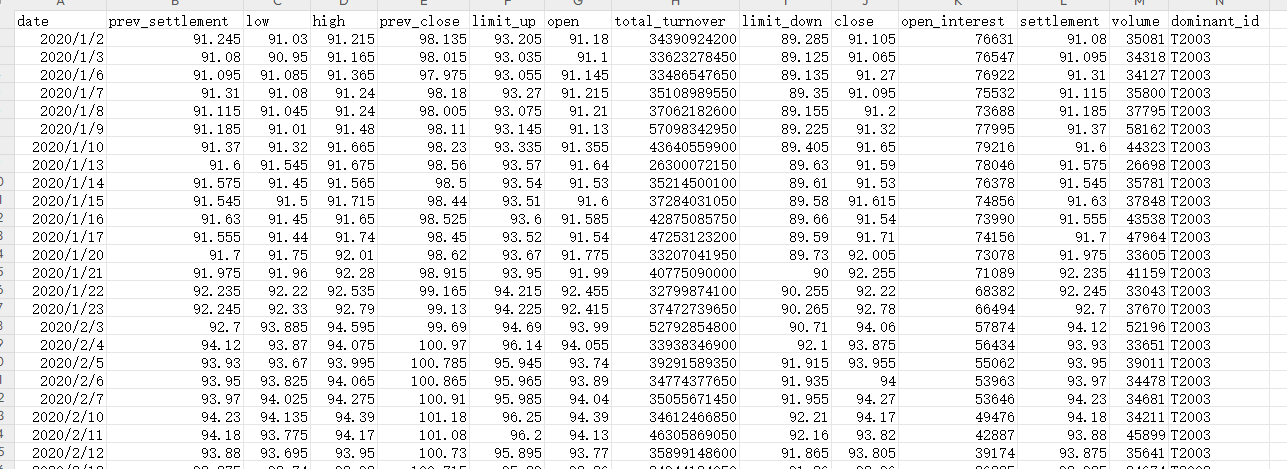
def plotResult(HQDf):
fig, axes = plt.subplots(4, 1, figsize=(16, 12))
HQDf.loc[:, ['base_balance', 'strategy_balance']].plot(ax=axes[0], title='净值曲线')
HQDf.loc[:, ['drawdown']].plot(ax=axes[1], title='回撤', kind='area')
HQDf.loc[:, ['pos']].plot(ax=axes[2], title='仓位', kind='area', stacked=False)
HQDf['empty'] = HQDf.close[HQDf.pos == 0]
HQDf['long'] = HQDf.close[HQDf.pos > 0]
HQDf['short'] = HQDf.close[HQDf.pos < 0]
HQDf.loc[:, ['long', 'short', 'empty']].plot(ax=axes[3], title='开平仓点位', color=["r", "g", "grey"])
plt.show()
def CTA(HQDf, loadBars, func, **kwargs):
HQDf['pos'] = np.nan
for idx, hq in HQDf.iterrows():
TradedHQDf = HQDf[:idx]
idx_num = TradedHQDf.shape[0]
if idx_num < loadBars:
continue
func(TradedHQDf, HQDf, idx, idx_num, **kwargs)
HQDf[:idx].pos = HQDf[:idx].pos.fillna(method='ffill')
HQDf, StatDf = CalculateResult(HQDf)
return HQDf, StatDf
def hypeFun(space, target):
"""
贝叶斯超参数优化
:param space: 参数空间
:param target: 优化目标
:return:
"""
def hyperparameter_tuning(params):
HQDf, StatDf = CTA(**params)
return {"loss": -StatDf[target], "status": STATUS_OK}
trials = Trials()
best = fmin(
fn=hyperparameter_tuning,
space=space,
algo=tpe.suggest,
max_evals=100,
trials=trials
)
print("Best: {}".format(best))
return trials, best
def doubleMa(*args, **kwargs):
TradedHQDf = args[0]
fast_ma = talib.SMA(TradedHQDf.close, timeperiod=kwargs['fast'])
fast_ma0 = fast_ma[-1]
fast_ma1 = fast_ma[-2]
slow_ma = talib.SMA(TradedHQDf.close, timeperiod=kwargs['slow'])
slow_ma0 = slow_ma[-1]
slow_ma1 = slow_ma[-2]
cross_over = fast_ma0 > slow_ma0 and fast_ma1 < slow_ma1
cross_below = fast_ma0 < slow_ma0 and fast_ma1 > slow_ma1
if cross_over:
setpos(1, *args)
elif cross_below:
setpos(-1, *args)
if __name__ == '__main__':
# 读取数据
HQDf = pd.read_csv('T888_1d.csv', index_col='date')
HQDf.index = pd.to_datetime(HQDf.index)
# 初始参数
ctaParas = {'fast': 5, 'slow': 10}
ResultTSDf, StatDf = CTA(HQDf, 30, doubleMa, **ctaParas)
plotResult(ResultTSDf)
# 定义贝叶斯搜索的空间
space = {
"HQDf": HQDf,
"loadBars": 40,
"func": doubleMa,
"fast": hp.quniform("fast", 3, 30, 1),
"slow": hp.quniform("slow", 5, 40, 1),
}
# 调用贝叶斯搜索,优化目标为夏普比率
trials, best = hypeFun(space, 'sharpe_ratio')
# 使用最佳参数进行回测
BestResultTSDf, BestStatDf = CTA(HQDf, 30, doubleMa, **best)
plotResult(BestResultTSDf)
输出结果:
优化前:
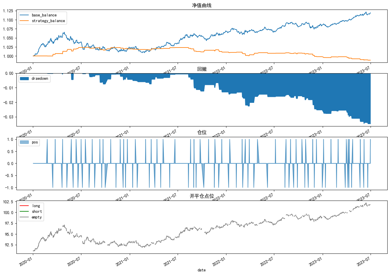
优化后:
可以看到优化后策略的净值曲线由下降变为上升趋势,且最大回撤也有降低;
OK,今天就学到这里!😊😊
相关链接
- 项目地址:AlgoQuant-CookBook
- 相关文档:专栏地址
- 作者主页:GISer Liu-CSDN博客

如果觉得我的文章对您有帮助,三连+关注便是对我创作的最大鼓励!或者一个star🌟也可以😂.


 1159
1159

 被折叠的 条评论
为什么被折叠?
被折叠的 条评论
为什么被折叠?
 到【灌水乐园】发言


