USPS数据集_kmeans使用总结

USPS数据集可视化

import h5py
hf = h5py.File('./data.h5', 'r')
X = np.asarray(hf.get('data'), dtype='float32')
X_train = (X - np.float32(127.5)) / np.float32(127.5)
y_train = np.asarray(hf.get('labels'), dtype='int32')
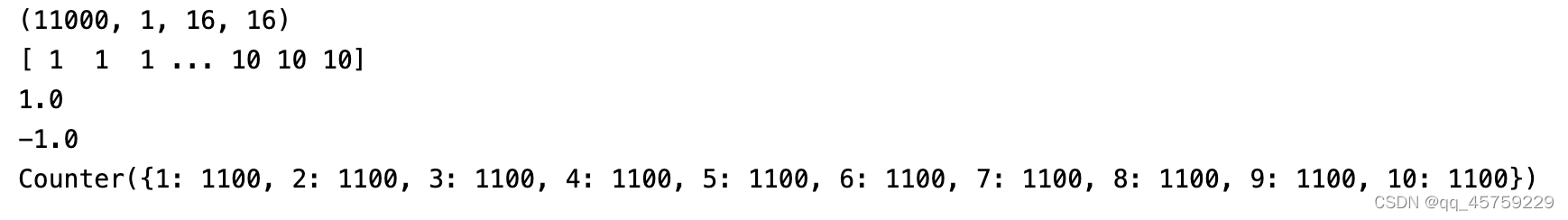
print(X_train.shape)
print(y_train)
print(np.max(X_train))
print(np.min(X_train))

from collections import Counter
print(Counter(y_train))
### 样本比例确实是1:1:1:1:1

%matplotlib inline
import matplotlib.pyplot as plt
import h5py
import numpy as np
filename=r"./data.h5"
f = h5py.File(filename,'r')   #打开h5文 件  
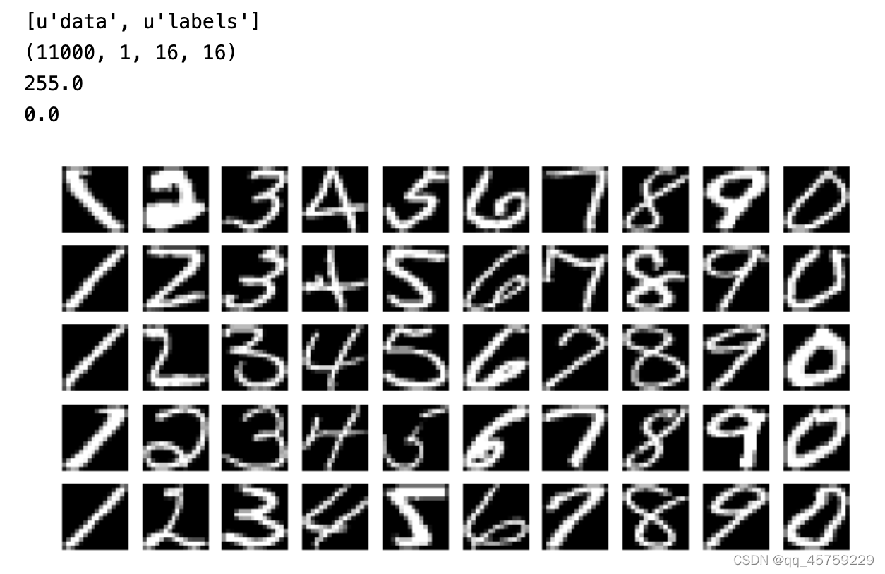
print(f.keys())                            #可以查看所有的主键  
dat = f['data'][:]                    #取出主键为data的所有的键值  
lab = f['labels'][:]
f.close() 
# 本来标签是1到10，现在把标签变成0-9

print(dat.shape)
print(np.max(dat[:]))
print(np.min(dat[:]))# 可以看到这个数据就是没有标准化的。全是0到255的值。
y_true_unique=np.unique(lab).astype(int)
y_tr=np.nonzero(lab[:, None] == y_true_unique)[1]

X_tr=np.reshape(dat,(11000,256))
#import ipdb
num_classes=10;
num_samples = 5
fig, ax = plt.subplots(num_samples, num_classes, sharex = True, sharey = True, figsize=(num_classes, num_samples))
for label in range(num_classes):
    class_idxs = np.where(y_tr == label)
    #ipdb.set_trace()
    for i, idx in enumerate(np.random.randint(0, class_idxs[0].shape[0], num_samples)):
        ax[i, label].imshow(X_tr[class_idxs[0][idx]].reshape([16, 16],order="F"), 'gray')
        ax[i, label].set_axis_off()

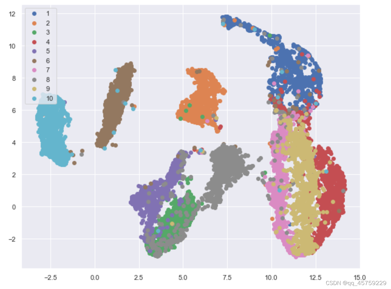
umap visulization

import umap
import h5py
import matplotlib.pyplot as plt
hf = h5py.File('./data.h5', 'r')
X = np.asarray(hf.get('data'), dtype='float32')
X_train = (X - np.float32(127.5)) / np.float32(127.5)
target = np.asarray(hf.get('labels'), dtype='int32')
X_mat=X_train.reshape((11000,256))
reducer=umap.UMAP(random_state=0)
X_transformed=reducer.fit_transform(X_mat)

fig=plt.figure(figsize=(10,8))
for label in np.unique(target):
    plt.scatter(X_transformed[label==target,0], X_transformed[label==target,1],label=label)
plt.legend(loc="upper left")
plt.show()

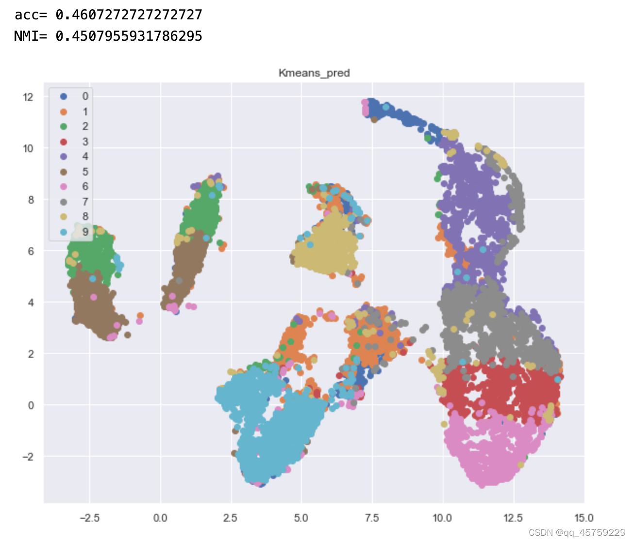
Kmeans的ACC,NMI

from scipy.optimize import linear_sum_assignment
def cluster_acc(y_true, y_pred):
    """
    This is code from original repository.
    Calculate clustering accuracy. Require scipy installed
    # Arguments
        y: true labels, numpy.array with shape `(n_samples,)`
        y_pred: predicted labels, numpy.array with shape `(n_samples,)`
    # Return
        accuracy, in [0,1]
    """
    y_true = y_true.astype(np.int64)
    assert y_pred.size == y_true.size
    D = max(y_pred.max(), y_true.max()) + 1
    w = np.zeros((D, D), dtype=np.int64)
    for i in range(y_pred.size):
        w[y_pred[i], y_true[i]] += 1

    ind = linear_sum_assignment(w.max() - w)

    accuracy = 0
    for idx in range(len(ind[0]) - 1):
        i = ind[0][idx]
        j = ind[1][idx]
        accuracy += w[i, j]
    accuracy = accuracy * 1.0 / y_pred.size
    return accuracy


from sklearn.cluster import KMeans

import h5py
hf = h5py.File('./data.h5', 'r')
X = np.asarray(hf.get('data'), dtype='float32')
X_train = (X - np.float32(127.5)) / np.float32(127.5)

X=np.reshape(X_train,(11000,256))
y_train = np.asarray(hf.get('labels'), dtype='int32')

kmeans = KMeans(n_clusters=10, init='k-means++', random_state=10)
# 这个和随机种子是有一定的差距的
pred_y = kmeans.fit_predict(X)

acc=cluster_acc(y_train,pred_y)
print("acc=",acc)
from sklearn import metrics
NMI=metrics.normalized_mutual_info_score(y_train, pred_y)
print("NMI=",NMI)

target=pred_y
fig=plt.figure(figsize=(10,8))
for label in np.unique(target):
    plt.scatter(X_transformed[label==target,0], X_transformed[label==target,1],label=label)
plt.legend(loc="upper left")
plt.title("Kmeans_pred")
plt.show()

混淆矩阵

案例学习

from sklearn.datasets import fetch_20newsgroups

categories = [
    'rec.motorcycles',
    'rec.sport.baseball',
    'comp.graphics',
    'sci.space',
    'talk.politics.mideast'
]

ng5 = fetch_20newsgroups(categories=categories, shuffle=True)

labels = ng5.target
documents = ng5.data

from sklearn.pipeline import Pipeline
from sklearn.feature_extraction.text import CountVectorizer
from sklearn.feature_extraction.text import TfidfTransformer
from sklearn.decomposition import TruncatedSVD
from sklearn.preprocessing import Normalizer

pipeline = Pipeline([
    ('vect', CountVectorizer()),
    ('tfidf', TfidfTransformer()),
    ('svd', TruncatedSVD()),
    ('normalizer', Normalizer())
])
pipeline.set_params(svd__n_components=300)
A = pipeline.fit_transform(documents)

kmeans使用教程

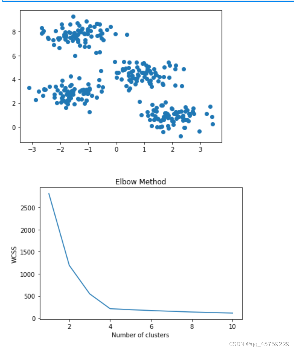
简单二维数据

import numpy as np
import pandas as pd
from matplotlib import pyplot as plt
from sklearn.datasets import make_blobs
from sklearn.cluster import KMeans
X, y = make_blobs(n_samples=300, centers=4, cluster_std=0.60, random_state=0)
# n_features=2是默认的
plt.scatter(X[:,0], X[:,1])
plt.show()
wcss = []
for i in range(1, 11):
    kmeans = KMeans(n_clusters=i, init='k-means++', max_iter=300, n_init=10, random_state=0)
    kmeans.fit(X)
    wcss.append(kmeans.inertia_)
plt.plot(range(1, 11), wcss)
plt.title('Elbow Method')
plt.xlabel('Number of clusters')
plt.ylabel('WCSS')
plt.show()

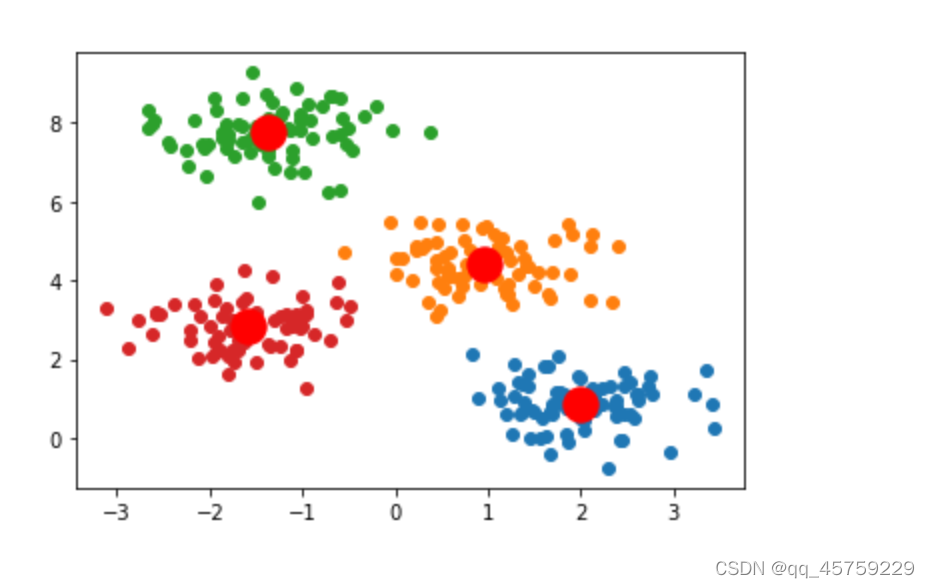
kmeans = KMeans(n_clusters=4, init='k-means++', max_iter=300, n_init=10, random_state=0)
pred_y = kmeans.fit_predict(X)
fig=plt.figure()
for label in np.unique(pred_y):
    plt.scatter(X[label==pred_y,0], X[label==pred_y,1],label=label)
plt.scatter(kmeans.cluster_centers_[:, 0], kmeans.cluster_centers_[:, 1], s=300, c='red')
plt.show()

高维例子

import numpy as np
import pandas as pd
import umap
from matplotlib import pyplot as plt
from sklearn.datasets import make_blobs
from sklearn.cluster import KMeans
X, y = make_blobs(n_samples=1000, n_features=50,centers=4, random_state=0)

target = y.copy()
X_mat=X.copy()
reducer=umap.UMAP(random_state=0)
X_transformed=reducer.fit_transform(X_mat)

fig=plt.figure(figsize=(10,8))
for label in np.unique(target):
    plt.scatter(X_transformed[label==target,0], X_transformed[label==target,1],label=label)
plt.legend(loc="upper left")
plt.show()

wcss = []
for i in range(1, 11):
    kmeans = KMeans(n_clusters=i, init='k-means++', max_iter=300, n_init=10, random_state=0)
    kmeans.fit(X)
    wcss.append(kmeans.inertia_)
plt.plot(range(1, 11), wcss)
plt.title('Elbow Method')
plt.xlabel('Number of clusters')
plt.ylabel('WCSS')
plt.show()