CS231n-assignment2-BatchNormalization

批标准化

使深度网络更容易训练的一种方法是使用更复杂的优化程序，如SGD+momentum、RMSProp或Adam。另一个策略是改变网络的架构，使其更容易训练
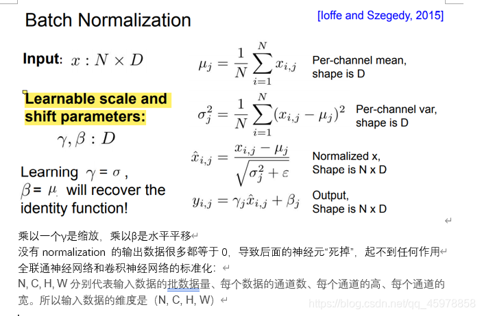
这个想法相对简单。当输入数据由零均值和单位方差的不相关特征组成时，机器学习方法往往工作得更好。在训练神经网络时，我们可以在将数据输入网络之前对其进行预处理，这将确保网络的第一层看到符合良好分布的数据。然而，即使我们对输入数据进行预处理，网络更深层次的激活也可能不再是去相关的，也不再具有零平均值或单位方差，因为它们是来自网络前面层的输出。更糟糕的是，在训练过程中，随着每一层权值的更新，网络每一层的特征分布也会发生变化。

深度神经网络内部特征分布的变化可能会使训练深度网络更加困难。为了解决这一问题，提出了在网络中插入批次归一化层。在训练时，批次归一化层使用小批数据来估计每个特征的平均值和标准差。这些估计的平均值和标准偏差然后被用来集中和标准化小批数据(mini batch)的特征。在训练期间保持这些平均值和标准差的运行平均值，并在测试时使用这些运行平均值来集中和标准化特征。

这种归一化策略可能会降低网络的表现能力，因为有时某些层可能具有非零均值或单位方差的特征是最优的。为此，批次归一化层包括每个特征维度的可学习的位移和尺度参数。

跟以前一样，准备工作走起
ln[1]:

import time
import numpy as np
import matplotlib.pyplot as plt
from cs231n.classifiers.fc_net import *
from cs231n.data_utils import get_CIFAR10_data
from cs231n.gradient_check import eval_numerical_gradient, eval_numerical_gradient_array
from cs231n.solver import Solver

#%matplotlib inline
plt.rcParams['figure.figsize'] = (10.0, 8.0) # set default size of plots
plt.rcParams['image.interpolation'] = 'nearest'
plt.rcParams['image.cmap'] = 'gray'

%load_ext autoreload
%autoreload 2

def rel_error(x, y):
    """ returns relative error """
    return np.max(np.abs(x - y) / (np.maximum(1e-8, np.abs(x) + np.abs(y))))

def print_mean_std(x,axis=0):
    print('  means: ', x.mean(axis=axis))
    print('  stds:  ', x.std(axis=axis))
    print()

ln[2]:

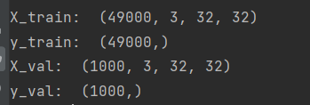
#载入数据
data = get_CIFAR10_data()
for k, v in data.items():
  print('%s: ' % k, v.shape)

在cs231n/layers.py文件中，完成batchnorm_forward，完成之后，运行以下操作来测试您的实现。

def batchnorm_forward(x, gamma, beta, bn_param):
    """
    Forward pass for batch normalization.

    During training the sample mean and (uncorrected) sample variance are
    computed from minibatch statistics and used to normalize the incoming data.
    During training we also keep an exponentially decaying running mean of the
    mean and variance of each feature, and these averages are used to normalize
    data at test-time.

    At each timestep we update the running averages for mean and variance using
    an exponential decay based on the momentum parameter:

    running_mean = momentum * running_mean + (1 - momentum) * sample_mean
    running_var = momentum * running_var + (1 - momentum) * sample_var

    Note that the batch normalization paper suggests a different test-time
    behavior: they compute sample mean and variance for each feature using a
    large number of training images rather than using a running average. For
    this implementation we have chosen to use running averages instead since
    they do not require an additional estimation step; the torch7
    implementation of batch normalization also uses running averages.

    Input:
    - x: Data of shape (N, D)
    - gamma: Scale parameter of shape (D,)
    - beta: Shift paremeter of shape (D,)
    - bn_param: Dictionary with the following keys:
      - mode: 'train' or 'test'; required
      - eps: Constant for numeric stability
      - momentum: Constant for running mean / variance.
      - running_mean: Array of shape (D,) giving running mean of features
      - running_var Array of shape (D,) giving running variance of features

    Returns a tuple of:
    - out: of shape (N, D)
    - cache: A tuple of values needed in the backward pass
    """
    mode = bn_param['mode']
    eps = bn_param.get('eps', 1e-5)
    momentum = bn_param.get('momentum', 0.9)
    layernorm = bn_param.get('layernorm', 0)

    N, D = x.shape
    running_mean = bn_param.get('running_mean', np.zeros(D, dtype=x.dtype))
    running_var = bn_param.get('running_var', np.zeros(D, dtype=x.dtype))

    out, cache = None, None
    if mode == 'train':
        #######################################################################
        # TODO: Implement the training-time forward pass for batch norm.      #
        # Use minibatch statistics to compute the mean and variance, use      #
        # these statistics to normalize the incoming data, and scale and      #
        # shift the normalized data using gamma and beta.                     #
        #                                                                     #
        # You should store the output in the variable out. Any intermediates  #
        # that you need for the backward pass should be stored in the cache   #
        # variable.                                                           #
        #                                                                     #
        # You should also use your computed sample mean and variance together #
        # with the momentum variable to update the running mean and running   #
        # variance, storing your result in the running_mean and running_var   #
        # variables.                                                          #
        #                                                                     #
        # Note that though you should be keeping track of the running         #
        # variance, you should normalize the data based on the standard       #
        # deviation (square root of variance) instead!                        # 
        # Referencing the original paper (https://arxiv.org/abs/1502.03167)   #
        # might prove to be helpful.                                          #
        #######################################################################
        mu = x.mean(axis=0)
        var = x.var(axis=0) + eps
        std = np.sqrt(var)
        z = (x - mu)/std
        out = gamma * z + beta
        if layernorm == 0:
           # running weighted average
           running_mean = momentum * running_mean + (1 - momentum) * mu
           running_var = momentum * running_var + (1 - momentum) * (std**2)
        # save values for backward call
        cache={'x':x,'mean':mu,'std':std,'gamma':gamma,'z':z,'var':var,'axis':layernorm}
        #######################################################################
        #                           END OF YOUR CODE                          #
        #######################################################################
    elif mode == 'test':
        #######################################################################
        # TODO: Implement the test-time forward pass for batch normalization. #
        # Use the running mean and variance to normalize the incoming data,   #
        # then scale and shift the normalized data using gamma and beta.      #
        # Store the result in the out variable.                               #
        #######################################################################
        out = gamma * (x - running_mean) / np.sqrt(running_var + eps) + beta
        #######################################################################
        #                          END OF YOUR CODE                           #
        #######################################################################
    else:
        raise ValueError('Invalid forward batchnorm mode "%s"' % mode)

    # Store the updated running means back into bn_param
    bn_param['running_mean'] = running_mean
    bn_param['running_var'] = running_var

    return out, cache

ln[3]:

np.random.seed(231)
N, D1, D2, D3 = 200, 50, 60, 3
X = np.random.randn(N, D1)
W1 = np.random.randn(D1, D2)
W2 = np.random.randn(D2, D3)
a = np.maximum(0, X.dot(W1)).dot(W2)

print('Before batch normalization:')
print_mean_std(a,axis=0)

gamma = np.ones((D3,))
beta = np.zeros((D3,))
# Means should be close to zero and stds close to one
print('After batch normalization (gamma=1, beta=0)')
a_norm, _ = batchnorm_forward(a, gamma, beta, {'mode': 'train'})
print_mean_std(a_norm,axis=0)

gamma = np.asarray([1.0, 2.0, 3.0])
beta = np.asarray([11.0, 12.0, 13.0])
# Now means should be close to beta and stds close to gamma
print('After batch normalization (gamma=', gamma, ', beta=', beta, ')')
a_norm, _ = batchnorm_forward(a, gamma, beta, {'mode': 'train'})
print_mean_std(a_norm,axis=0)

check the test-time forwardpass:
ln[4]:

np.random.seed(231)
N, D1, D2, D3 = 200, 50, 60, 3
W1 = np.random.randn(D1, D2)
W2 = np.random.randn(D2, D3)

bn_param = {'mode': 'train'}
gamma = np.ones(D3)
beta = np.zeros(D3)

for t in range(50):
  X = np.random.randn(N, D1)
  a = np.maximum(0, X.dot(W1)).dot(W2)
  batchnorm_forward(a, gamma, beta, bn_param)

bn_param['mode'] = 'test'
X = np.random.randn(N, D1)
a = np.maximum(0, X.dot(W1)).dot(W2)
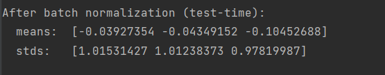
a_norm, _ = batchnorm_forward(a, gamma, beta, bn_param)

# Means should be close to zero and stds close to one, but will be
# noisier than training-time forward passes.
print('After batch normalization (test-time):')
print_mean_std(a_norm,axis=0)

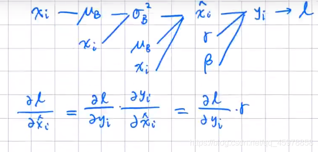
现在在函数batchnorm_backward中实现批标准化的向后传递。

要推导向后传递，您应该写出通过每个中间节点进行批标准化和backprop的计算图。一些中间程序可能有多个传出分支;确保在向后通过这些分支累加渐变。

以此类推

def batchnorm_backward(dout, cache):
    """
    Backward pass for batch normalization.

    For this implementation, you should write out a computation graph for
    batch normalization on paper and propagate gradients backward through
    intermediate nodes.

    Inputs:
    - dout: Upstream derivatives, of shape (N, D)
    - cache: Variable of intermediates from batchnorm_forward.

    Returns a tuple of:
    - dx: Gradient with respect to inputs x, of shape (N, D)
    - dgamma: Gradient with respect to scale parameter gamma, of shape (D,)
    - dbeta: Gradient with respect to shift parameter beta, of shape (D,)
    """
    dx, dgamma, dbeta = None, None, None
    ###########################################################################
    # TODO: Implement the backward pass for batch normalization. Store the    #
    # results in the dx, dgamma, and dbeta variables.                         #
    # Referencing the original paper (https://arxiv.org/abs/1502.03167)       #
    # might prove to be helpful.                                              #
    ###########################################################################
    dbeta = dout.sum(axis=cache['axis'])
    dgamma = np.sum(dout * cache['z'], axis=cache['axis'])

    N = 1.0 * dout.shape[0]
    dfdz = dout * cache['gamma']                                    #[NxD]
    dudx = 1/N                                                      #[NxD]
    dvdx = 2/N * (cache['x'] - cache['mean'])                       #[NxD] 
    dzdx = 1 / cache['std']                                         #[NxD]
    dzdu = -1 / cache['std']                                        #[1xD]
    dzdv = -0.5*(cache['var']**-1.5)*(cache['x']-cache['mean'])     #[NxD]
    dvdu = -2/N * np.sum(cache['x'] - cache['mean'], axis=0)        #[1xD]

    dx = dfdz*dzdx + np.sum(dfdz*dzdu,axis=0)*dudx + \
         np.sum(dfdz*dzdv,axis=0)*(dvdx+dvdu*dudx)
    ###########################################################################
    #                             END OF YOUR CODE                            #
    ###########################################################################

    return dx, dgamma, dbeta

ln[5]:

np.random.seed(231)
N, D = 4, 5
x = 5 * np.random.randn(N, D) + 12
gamma = np.random.randn(D)
beta = np.random.randn(D)
dout = np.random.randn(N, D)

bn_param = {'mode': 'train'}
fx = lambda x: batchnorm_forward(x, gamma, beta, bn_param)[0]
fg = lambda a: batchnorm_forward(x, a, beta, bn_param)[0]
fb = lambda b: batchnorm_forward(x, gamma, b, bn_param)[0]

dx_num = eval_numerical_gradient_array(fx, x, dout)
da_num = eval_numerical_gradient_array(fg, gamma.copy(), dout)
db_num = eval_numerical_gradient_array(fb, beta.copy(), dout)

_, cache = batchnorm_forward(x, gamma, beta, bn_param)
dx, dgamma, dbeta = batchnorm_backward(dout, cache)

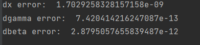
#You should expect to see relative errors between 1e-13 and 1e-8
print('dx error: ', rel_error(dx_num, dx))
print('dgamma error: ', rel_error(da_num, dgamma))
print('dbeta error: ', rel_error(db_num, dbeta))

在函数batchnorm_backward_alt中实现简化的批标准化向后传递
就是在上面做一些改进加快计算

def batchnorm_backward_alt(dout, cache):
    """
    Alternative backward pass for batch normalization.

    For this implementation you should work out the derivatives for the batch
    normalizaton backward pass on paper and simplify as much as possible. You
    should be able to derive a simple expression for the backward pass. 
    See the jupyter notebook for more hints.
     
    Note: This implementation should expect to receive the same cache variable
    as batchnorm_backward, but might not use all of the values in the cache.

    Inputs / outputs: Same as batchnorm_backward
    """
    dx, dgamma, dbeta = None, None, None
    ###########################################################################
    # TODO: Implement the backward pass for batch normalization. Store the    #
    # results in the dx, dgamma, and dbeta variables.                         #
    #                                                                         #
    # After computing the gradient with respect to the centered inputs, you   #
    # should be able to compute gradients with respect to the inputs in a     #
    # single statement; our implementation fits on a single 80-character line.#
    ###########################################################################
    dbeta = dout.sum(axis=cache['axis'])
    dgamma = np.sum(dout * cache['z'], axis=cache['axis'])

    N = dout.shape[0]
    z = cache['z']
    dfdz = dout * cache['gamma']                                    #[NxD]
    dfdz_sum = np.sum(dfdz,axis=0)                                  #[1xD]
    dx = dfdz - dfdz_sum/N - np.sum(dfdz * z,axis=0) * z/N          #[NxD]
    dx /= cache['std']
    ###########################################################################
    #                             END OF YOUR CODE                            #
    ###########################################################################

    return dx, dgamma, dbeta

ln[6]:

np.random.seed(231)
N, D = 100, 500
x = 5 * np.random.randn(N, D) + 120
gamma = np.random.randn(D)
beta = np.random.randn(D)
dout = np.random.randn(N, D)

bn_param = {'mode': 'train'}
out, cache = batchnorm_forward(x, gamma, beta, bn_param)

t1 = time.time()
dx1, dgamma1, dbeta1 = batchnorm_backward(dout, cache)
t2 = time.time()
dx2, dgamma2, dbeta2 = batchnorm_backward_alt(dout, cache)
t3 = time.time()

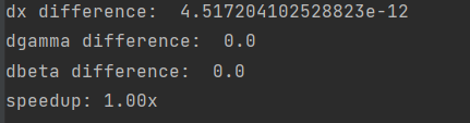
print('dx difference: ', rel_error(dx1, dx2))
print('dgamma difference: ', rel_error(dgamma1, dgamma2))
print('dbeta difference: ', rel_error(dbeta1, dbeta2))
print('speedup: %.2fx' % ((t2 - t1) / (t3 - t2)))

批量标准化的全连接网络

现在您已经有了批标准化的工作实现，回到文件cs231n/classifiers/fc_net.py中的fulllyconnectednet。修改您的实现以添加批标准化。

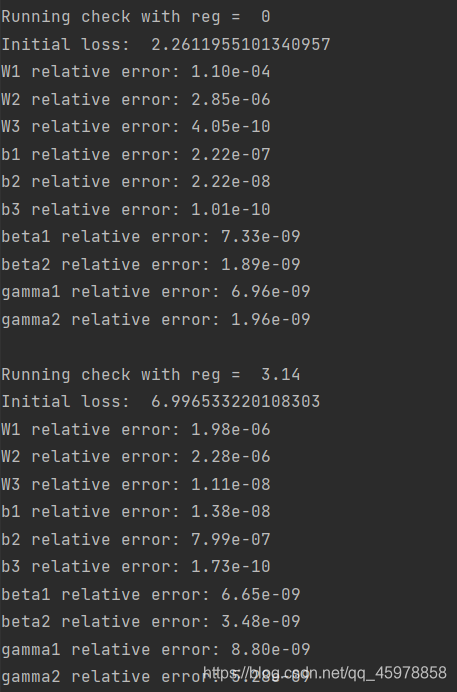
具体来说，当在构造函数中将标准化标志设置为“batchnorm”时，您应该在每个ReLU非线性之前插入一个批标准化层。来自网络最后一层的输出不应该被规范化。完成之后，运行以下命令对实现进行渐变检查。

ln[7]:

np.random.seed(231)
N, D, H1, H2, C = 2, 15, 20, 30, 10
X = np.random.randn(N, D)
y = np.random.randint(C, size=(N,))

# You should expect losses between 1e-4~1e-10 for W, 
# losses between 1e-08~1e-10 for b,
# and losses between 1e-08~1e-09 for beta and gammas.
for reg in [0, 3.14]:
  print('Running check with reg = ', reg)
  model = FullyConnectedNet([H1, H2], input_dim=D, num_classes=C,
                            reg=reg, weight_scale=5e-2, dtype=np.float64,
                            normalization='batchnorm')

  loss, grads = model.loss(X, y)
  print('Initial loss: ', loss)

  for name in sorted(grads):
    f = lambda _: model.loss(X, y)[0]
    grad_num = eval_numerical_gradient(f, model.params[name], verbose=False, h=1e-5)
    print('%s relative error: %.2e' % (name, rel_error(grad_num, grads[name])))
  if reg == 0: print()

运行以下命令，在1000个训练示例的子集上训练一个六层网络,一个进行批标准化，一个不进行
In[8]:

np.random.seed(231)
# Try training a very deep net with batchnorm
hidden_dims = [100, 100, 100, 100, 100]

num_train = 1000
small_data = {
  'X_train': data['X_train'][:num_train],
  'y_train': data['y_train'][:num_train],
  'X_val': data['X_val'],
  'y_val': data['y_val'],
}

weight_scale = 2e-2
bn_model = FullyConnectedNet(hidden_dims, weight_scale=weight_scale, normalization='batchnorm')
model = FullyConnectedNet(hidden_dims, weight_scale=weight_scale, normalization=None)

bn_solver = Solver(bn_model, small_data,
                num_epochs=10, batch_size=50,
                update_rule='adam',
                optim_config={
                  'learning_rate': 1e-3,
                },
                verbose=True,print_every=20)
bn_solver.train()

solver = Solver(model, small_data,
                num_epochs=10, batch_size=50,
                update_rule='adam',
                optim_config={
                  'learning_rate': 1e-3,
                },
                verbose=True, print_every=20)
solver.train()

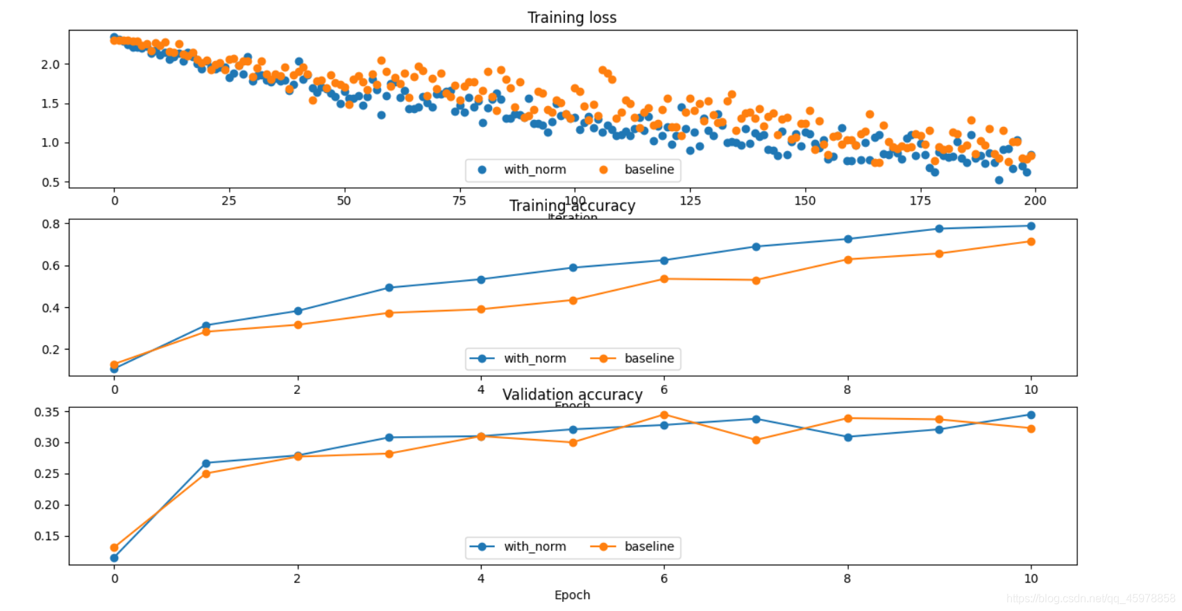
运行下面的程序来可视化上面训练的两个网络的结果。您应该发现，使用批处理规范化有助于网络更快地收敛
In[9]:

def plot_training_history(title, label, baseline, bn_solvers, plot_fn, bl_marker='.', bn_marker='.', labels=None):
    """utility function for plotting training history"""
    plt.title(title)
    plt.xlabel(label)
    bn_plots = [plot_fn(bn_solver) for bn_solver in bn_solvers]
    bl_plot = plot_fn(baseline)
    num_bn = len(bn_plots)
    for i in range(num_bn):
        label='with_norm'
        if labels is not None:
            label += str(labels[i])
        plt.plot(bn_plots[i], bn_marker, label=label)
    label='baseline'
    if labels is not None:
        label += str(labels[0])
    plt.plot(bl_plot, bl_marker, label=label)
    plt.legend(loc='lower center', ncol=num_bn+1) 

    
plt.subplot(3, 1, 1)
plot_training_history('Training loss','Iteration', solver, [bn_solver], \
                      lambda x: x.loss_history, bl_marker='o', bn_marker='o')
plt.subplot(3, 1, 2)
plot_training_history('Training accuracy','Epoch', solver, [bn_solver], \
                      lambda x: x.train_acc_history, bl_marker='-o', bn_marker='-o')
plt.subplot(3, 1, 3)
plot_training_history('Validation accuracy','Epoch', solver, [bn_solver], \
                      lambda x: x.val_acc_history, bl_marker='-o', bn_marker='-o')

plt.gcf().set_size_inches(15, 15)
plt.show()

批处理规范化和初始化

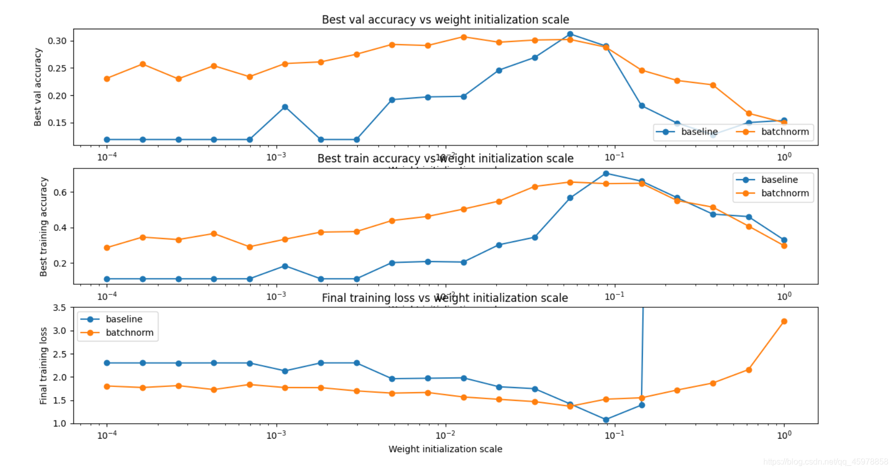
现在我们将进行一个小实验来研究批归一化和权值初始化的相互作用。

第一个单元将训练8层网络，使用不同的尺度进行权值初始化。第二层将训练准确性、验证集准确性和训练损失作为权重初始化尺度的函数绘制。
In[10]:

np.random.seed(231)
# Try training a very deep net with batchnorm
hidden_dims = [50, 50, 50, 50, 50, 50, 50]
num_train = 1000
small_data = {
  'X_train': data['X_train'][:num_train],
  'y_train': data['y_train'][:num_train],
  'X_val': data['X_val'],
  'y_val': data['y_val'],
}

bn_solvers_ws = {}
solvers_ws = {}
weight_scales = np.logspace(-4, 0, num=20)
for i, weight_scale in enumerate(weight_scales):
  print('Running weight scale %d / %d' % (i + 1, len(weight_scales)))
  bn_model = FullyConnectedNet(hidden_dims, weight_scale=weight_scale, normalization='batchnorm')
  model = FullyConnectedNet(hidden_dims, weight_scale=weight_scale, normalization=None)

  bn_solver = Solver(bn_model, small_data,
                  num_epochs=10, batch_size=50,
                  update_rule='adam',
                  optim_config={
                    'learning_rate': 1e-3,
                  },
                  verbose=False, print_every=200)
  bn_solver.train()
  bn_solvers_ws[weight_scale] = bn_solver

  solver = Solver(model, small_data,
                  num_epochs=10, batch_size=50,
                  update_rule='adam',
                  optim_config={
                    'learning_rate': 1e-3,
                  },
                  verbose=False, print_every=200)
  solver.train()
  solvers_ws[weight_scale] = solver

In[11]:

best_train_accs, bn_best_train_accs = [], []
best_val_accs, bn_best_val_accs = [], []
final_train_loss, bn_final_train_loss = [], []

for ws in weight_scales:
  best_train_accs.append(max(solvers_ws[ws].train_acc_history))
  bn_best_train_accs.append(max(bn_solvers_ws[ws].train_acc_history))
  
  best_val_accs.append(max(solvers_ws[ws].val_acc_history))
  bn_best_val_accs.append(max(bn_solvers_ws[ws].val_acc_history))
  
  final_train_loss.append(np.mean(solvers_ws[ws].loss_history[-100:]))
  bn_final_train_loss.append(np.mean(bn_solvers_ws[ws].loss_history[-100:]))
  
plt.subplot(3, 1, 1)
plt.title('Best val accuracy vs weight initialization scale')
plt.xlabel('Weight initialization scale')
plt.ylabel('Best val accuracy')
plt.semilogx(weight_scales, best_val_accs, '-o', label='baseline')
plt.semilogx(weight_scales, bn_best_val_accs, '-o', label='batchnorm')
plt.legend(ncol=2, loc='lower right')

plt.subplot(3, 1, 2)
plt.title('Best train accuracy vs weight initialization scale')
plt.xlabel('Weight initialization scale')
plt.ylabel('Best training accuracy')
plt.semilogx(weight_scales, best_train_accs, '-o', label='baseline')
plt.semilogx(weight_scales, bn_best_train_accs, '-o', label='batchnorm')
plt.legend()

plt.subplot(3, 1, 3)
plt.title('Final training loss vs weight initialization scale')
plt.xlabel('Weight initialization scale')
plt.ylabel('Final training loss')
plt.semilogx(weight_scales, final_train_loss, '-o', label='baseline')
plt.semilogx(weight_scales, bn_final_train_loss, '-o', label='batchnorm')
plt.legend()
plt.gca().set_ylim(1.0, 3.5)

plt.gcf().set_size_inches(15, 15)
plt.show()

内联问题1:
描述这个实验的结果。权重初始化的规模如何影响有/没有批量规范化的模型，为什么?
第二个图显示了消失的梯度(小初始权值)的问题。baseline模型对这个问题非常敏感(精度非常低)，因此很难找到正确的W。对于本例，baseline在权重为1e-1时获得最佳结果。另一方面，我们可以看到批标准化模型对权值初始化的敏感性较低，因为在所有不同的权值尺度下，它的正确率在30%左右。
第一个图与第二个图类似。主要的区别是，第一个图显示我们的模型过拟合，除此之外，我们可以看到，批标准化模型我们获得了比baseline模型更好的结果，这是因为batch normalization有正则化特性。
第三个图描述了爆炸式梯度的问题，这在baseline模型中非常明显，重量尺度值大于1e-1。然而，批标准化模型没有这个问题。
通常，使用批处理归一化，我们可以避免梯度消失和爆炸的问题，因为它归一化每一个仿射层(xW+b)，避免非常大/小的值。此外，它的正则化特性允许减少过拟合。

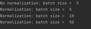
批规范化和批大小

现在我们将进行一个小实验来研究批标准化和批大小的相互作用。

第一个单元将使用不同的批大小训练有批标准化和没有批标准化的6层网络。第二层将绘制训练准确性和验证集准确性随时间的变化。
In[12]:

def run_batchsize_experiments(normalization_mode):
    np.random.seed(231)
    # Try training a very deep net with batchnorm
    hidden_dims = [100, 100, 100, 100, 100]
    num_train = 1000
    small_data = {
      'X_train': data['X_train'][:num_train],
      'y_train': data['y_train'][:num_train],
      'X_val': data['X_val'],
      'y_val': data['y_val'],
    }
    n_epochs=10
    weight_scale = 2e-2
    batch_sizes = [5,10,50]
    lr = 10**(-3.5)
    solver_bsize = batch_sizes[0]

    print('No normalization: batch size = ',solver_bsize)
    model = FullyConnectedNet(hidden_dims, weight_scale=weight_scale, normalization=None)
    solver = Solver(model, small_data,
                    num_epochs=n_epochs, batch_size=solver_bsize,
                    update_rule='adam',
                    optim_config={
                      'learning_rate': lr,
                    },
                    verbose=False)
    solver.train()
    
    bn_solvers = []
    for i in range(len(batch_sizes)):
        b_size=batch_sizes[i]
        print('Normalization: batch size = ',b_size)
        bn_model = FullyConnectedNet(hidden_dims, weight_scale=weight_scale, normalization=normalization_mode)
        bn_solver = Solver(bn_model, small_data,
                        num_epochs=n_epochs, batch_size=b_size,
                        update_rule='adam',
                        optim_config={
                          'learning_rate': lr,
                        },
                        verbose=False)
        bn_solver.train()
        bn_solvers.append(bn_solver)
        
    return bn_solvers, solver, batch_sizes

batch_sizes = [5,10,50]
bn_solvers_bsize, solver_bsize, batch_sizes = run_batchsize_experiments('batchnorm')

ln[13]:

plt.subplot(2, 1, 1)
plot_training_history('Training accuracy (Batch Normalization)','Epoch', solver_bsize, bn_solvers_bsize, \
                      lambda x: x.train_acc_history, bl_marker='-^', bn_marker='-o', labels=batch_sizes)
plt.subplot(2, 1, 2)
plot_training_history('Validation accuracy (Batch Normalization)','Epoch', solver_bsize, bn_solvers_bsize, \
                      lambda x: x.val_acc_history, bl_marker='-^', bn_marker='-o', labels=batch_sizes)

plt.gcf().set_size_inches(15, 10)
plt.show()

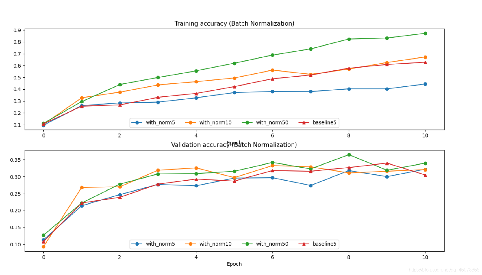
内联问题2:
描述这个实验的结果。这对批标准化和批大小之间的关系意味着什么?为什么会观察到这种关系?
由结果可以看出，批大小直接影响批归一化的性能(批大小越小越差)。当使用非常小的批大小时，甚至baseline模型的性能也优于批规范模型。出现这个问题是因为当我们计算一批统计数据时，即平均值和方差，我们试图找到整个数据集的统计数据的近似值。因此，在小批量的情况下，这些统计数据可能会非常嘈杂。另一方面，在批量较大的情况下，我们可以得到更好的近似。

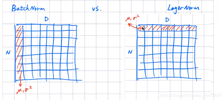
层标准化

批标准化已经被证明在使网络更容易训练方面是有效的，但是对批大小的依赖使得它在复杂的网络中用处不大，因为硬件限制对输入批大小有限制。

为了缓解这一问题，已经提出了几种替代批标准化的方法;其中一种技术就是图层标准化。我们不是对批处理进行规范化，而是对特性进行规范化。换句话说，当使用Layer Normalization时，对应于单个数据点的每个特征向量都是基于该特征向量中所有项的和进行标准化的。

内联问题3:
这些数据预处理步骤中哪一个类似于批处理的标准化，哪一个类似于层的标准化?
1.缩放数据集中的每个图像，使图像中每一行像素的RGB通道之和为1。
2.缩放数据集中的每个图像，使图像中所有像素的RGB通道之和为1。
3.从数据集中的每个图像减去数据集的平均图像。
4.根据给定的阈值将所有RGB值设置为0或1。
当我们考虑:均值= 0,beta参数= 0(此时我们有gammax/std，其中std=sqrt(sum(x^2)))和gamma=x/std),第2项类似于层标准化。
当我们考虑批量大小=数据集的大小，gamma参数=标准偏差和beta参数= 0时，3类似于批标准化。因此，批标准化的结果将是std(x-mean)/std + 0 = x-mean。

层标准化:实现

这个步骤应该相对简单，因为从概念上讲，它的实现几乎与批标准化的实现相同。一个显著的区别是，对于层标准化，我们不跟踪运动时刻，测试阶段与训练阶段是相同的，其中的平均值和方差是直接计算每个数据点。

你需要做的是:

在cs231n/layers.py中，在函数layernorm_backward中实现层标准化的前向传递。
在cs231n/layers.py中，在函数layernorm_backward中实现层标准化的向后传递。
修改cs231n/classifiers/fc_net.py，向fullyconnectednet添加层标准化。当在构造函数中将标准化标志设置为“layernorm”时，你应该在每个ReLU非线性之前插入一个层标准化层。

所以在层标准化中，将x转置即可跟批标准化一样

def layernorm_forward(x, gamma, beta, ln_param):
    """
    Forward pass for layer normalization.

    During both training and test-time, the incoming data is normalized per data-point,
    before being scaled by gamma and beta parameters identical to that of batch normalization.
    
    Note that in contrast to batch normalization, the behavior during train and test-time for
    layer normalization are identical, and we do not need to keep track of running averages
    of any sort.

    Input:
    - x: Data of shape (N, D)
    - gamma: Scale parameter of shape (D,)
    - beta: Shift paremeter of shape (D,)
    - ln_param: Dictionary with the following keys:
        - eps: Constant for numeric stability

    Returns a tuple of:
    - out: of shape (N, D)
    - cache: A tuple of values needed in the backward pass
    """
    out, cache = None, None
    eps = ln_param.get('eps', 1e-5)
    ###########################################################################
    # TODO: Implement the training-time forward pass for layer norm.          #
    # Normalize the incoming data, and scale and  shift the normalized data   #
    #  using gamma and beta.                                                  #
    # HINT: this can be done by slightly modifying your training-time         #
    # implementation of  batch normalization, and inserting a line or two of  #
    # well-placed code. In particular, can you think of any matrix            #
    # transformations you could perform, that would enable you to copy over   #
    # the batch norm code and leave it almost unchanged?                      #
    ###########################################################################
    ln_param['mode'] = 'train' # same as batch norm in train mode
    ln_param['layernorm'] = 1
    # transpose x, gamma and beta
    out, cache = batchnorm_forward(x.T, gamma.reshape(-1,1),
                                   beta.reshape(-1,1), ln_param)
    # transpose output to get original dims
    out = out.T
    ###########################################################################
    #                             END OF YOUR CODE                            #
    ###########################################################################
    return out, cache


def layernorm_backward(dout, cache):
    """
    Backward pass for layer normalization.

    For this implementation, you can heavily rely on the work you've done already
    for batch normalization.

    Inputs:
    - dout: Upstream derivatives, of shape (N, D)
    - cache: Variable of intermediates from layernorm_forward.

    Returns a tuple of:
    - dx: Gradient with respect to inputs x, of shape (N, D)
    - dgamma: Gradient with respect to scale parameter gamma, of shape (D,)
    - dbeta: Gradient with respect to shift parameter beta, of shape (D,)
    """
    dx, dgamma, dbeta = None, None, None
    ###########################################################################
    # TODO: Implement the backward pass for layer norm.                       #
    #                                                                         #
    # HINT: this can be done by slightly modifying your training-time         #
    # implementation of batch normalization. The hints to the forward pass    #
    # still apply!                                                            #
    ###########################################################################
    # transpose dout because we transposed original input, x, in forward call
    dx, dgamma, dbeta = batchnorm_backward_alt(dout.T, cache)
    # transpose gradients w.r.t. input, x, to their original dims
    dx = dx.T
    ###########################################################################
    #                             END OF YOUR CODE                            #
    ###########################################################################
    return dx, dgamma, dbeta

向前传递：
ln[14]:

np.random.seed(231)
N, D1, D2, D3 =4, 50, 60, 3
X = np.random.randn(N, D1)
W1 = np.random.randn(D1, D2)
W2 = np.random.randn(D2, D3)
a = np.maximum(0, X.dot(W1)).dot(W2)

print('Before layer normalization:')
print_mean_std(a,axis=1)

gamma = np.ones(D3)
beta = np.zeros(D3)
# Means should be close to zero and stds close to one
print('After layer normalization (gamma=1, beta=0)')
a_norm, _ = layernorm_forward(a, gamma, beta, {'mode': 'train'})
print_mean_std(a_norm,axis=1)

gamma = np.asarray([3.0,3.0,3.0])
beta = np.asarray([5.0,5.0,5.0])
# Now means should be close to beta and stds close to gamma
print('After layer normalization (gamma=', gamma, ', beta=', beta, ')')
a_norm, _ = layernorm_forward(a, gamma, beta, {'mode': 'train'})
print_mean_std(a_norm,axis=1)

检查向后传递的梯度
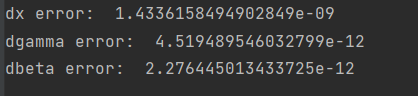
ln[15]:

np.random.seed(231)
N, D = 4, 5
x = 5 * np.random.randn(N, D) + 12
gamma = np.random.randn(D)
beta = np.random.randn(D)
dout = np.random.randn(N, D)

ln_param = {}
fx = lambda x: layernorm_forward(x, gamma, beta, ln_param)[0]
fg = lambda a: layernorm_forward(x, a, beta, ln_param)[0]
fb = lambda b: layernorm_forward(x, gamma, b, ln_param)[0]

dx_num = eval_numerical_gradient_array(fx, x, dout)
da_num = eval_numerical_gradient_array(fg, gamma.copy(), dout)
db_num = eval_numerical_gradient_array(fb, beta.copy(), dout)

_, cache = layernorm_forward(x, gamma, beta, ln_param)
dx, dgamma, dbeta = layernorm_backward(dout, cache)

#You should expect to see relative errors between 1e-12 and 1e-8
print('dx error: ', rel_error(dx_num, dx))
print('dgamma error: ', rel_error(da_num, dgamma))
print('dbeta error: ', rel_error(db_num, dbeta))

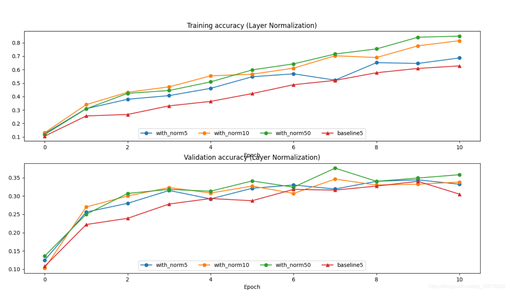
层标准化和批大小

现在我们将使用层标准化而不是批标准化来运行之前的批大小实验。与之前的实验相比，您应该会看到批大小对训练历史的影响明显更小!
ln[16]:

ln_solvers_bsize, solver_bsize, batch_sizes = run_batchsize_experiments('layernorm')

plt.subplot(2, 1, 1)
plot_training_history('Training accuracy (Layer Normalization)','Epoch', solver_bsize, ln_solvers_bsize, \
                      lambda x: x.train_acc_history, bl_marker='-^', bn_marker='-o', labels=batch_sizes)
plt.subplot(2, 1, 2)
plot_training_history('Validation accuracy (Layer Normalization)','Epoch', solver_bsize, ln_solvers_bsize, \
                      lambda x: x.val_acc_history, bl_marker='-^', bn_marker='-o', labels=batch_sizes)

plt.gcf().set_size_inches(15, 10)
plt.show()

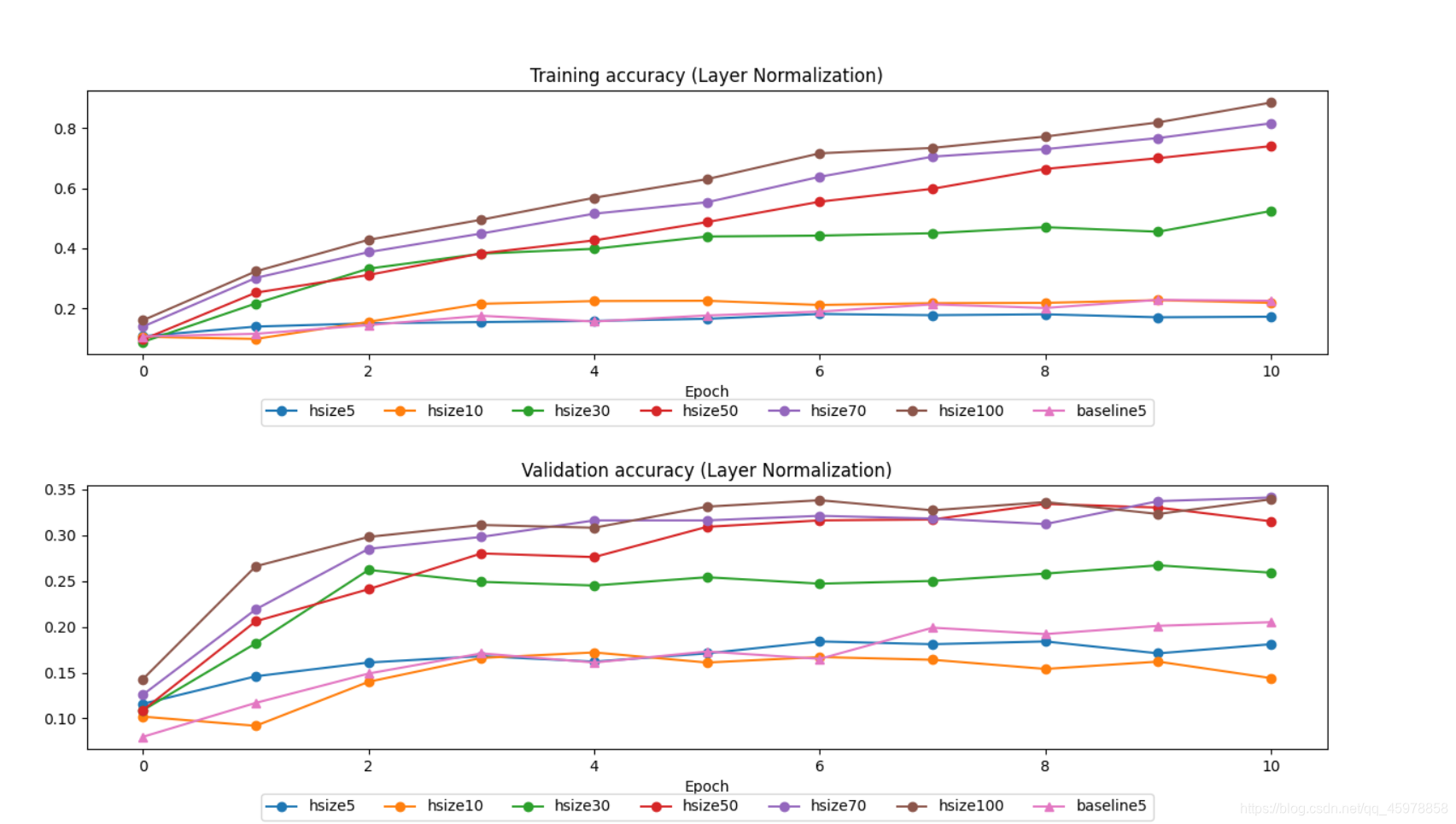
内联问题4:
什么时候层标准化可能不能很好地工作，为什么?
1.在一个非常深的网络中使用它
2.特征尺寸很小的
3.具有高正规化项
答:
1.[不正确]在前面的例子中，网络有五层，可以认为是一个深层网络。因此，在深度网络中使用层标准化是正确的。
2.[正确]特征的小维度会影响层标准化的性能。这个问题非常类似于小批量批量标准化的问题，因为在层标准化中，我们是根据隐含单元的数量来计算统计数据的，这些隐含单元代表了网络正在学习的特征。因此，隐藏尺寸越小，层标准化中使用的统计量噪声越大。
3.[正确]有一个高的正则化项会影响层标准化的性能。一般来说，当正则项非常高时，模型学习非常简单的函数(欠拟合)。
在下面可以看到显示具有不同隐藏大小和正则化值的层标准化性能的测试。

层标准化和隐藏大小

我们将运行一个实验，改变隐藏的大小值与层标准化。
ln[17]:

def run_hiddensize_experiments(normalization_mode):
    np.random.seed(231)
    # Try training network with different hidden sizes
    hidden_size = [5,10,30,50,70,100]
    solver_hidden_dims = [10, 10, 10, 10]
    num_train = 1000
    small_data = {
      'X_train': data['X_train'][:num_train],
      'y_train': data['y_train'][:num_train],
      'X_val': data['X_val'],
      'y_val': data['y_val'],
    }
    n_epochs=10
    weight_scale = 2e-2
    lr = 10**(-3.5)
    
    print('No normalization: hidden_sizes = ', hidden_size[0])
    model = FullyConnectedNet(solver_hidden_dims, weight_scale=weight_scale, normalization=None)
    solver = Solver(model, small_data,
                    num_epochs=n_epochs, batch_size=50,
                    update_rule='adam',
                    optim_config={
                      'learning_rate': lr,
                    },
                    verbose=False)
    solver.train()
    
    bn_solvers = []
    for i in range(len(hidden_size)):
        print('Normalization: hidden sizes = ', hidden_size[i])
        hidden_dims = [ hidden_size[i] for j in range(4)]
        bn_model = FullyConnectedNet(hidden_dims, weight_scale=weight_scale, normalization=normalization_mode)
        bn_solver = Solver(bn_model, small_data,
                        num_epochs=n_epochs, batch_size=50,
                        update_rule='adam',
                        optim_config={
                          'learning_rate': lr,
                        },
                        verbose=False)
        bn_solver.train()
        bn_solvers.append(bn_solver)
        
    return bn_solvers, solver, hidden_size

# Run model
ln_solvers_hsize, solver_hsize, hidden_size = run_hiddensize_experiments('layernorm')

ln[18]:

# Plot results
def plot_training_history2(title, label, baseline, bn_solvers, plot_fn, bl_marker='.', bn_marker='.',labels=None, label_prefix= '-'):
    """utility function for plotting training history"""
    plt.title(title)
    plt.xlabel(label)
    bn_plots = [plot_fn(bn_solver) for bn_solver in bn_solvers]
    bl_plot = plot_fn(baseline)
    num_bn = len(bn_plots)
    for i in range(num_bn):
        label=label_prefix
        if labels is not None:
            label += str(labels[i]) #str("%.4lf" %labels[i])
        plt.plot(bn_plots[i], bn_marker, label=label)
    label='baseline'
    if labels is not None:
        label += str(labels[0])
    plt.plot(bl_plot, bl_marker, label=label)
    plt.legend(loc='lower center', ncol=num_bn+1, bbox_to_anchor=(0.5, -0.3))

plt.subplot(2, 1, 1)
plot_training_history2('Training accuracy (Layer Normalization)','Epoch', solver_hsize, ln_solvers_hsize, \
                      lambda x: x.train_acc_history, bl_marker='-^', bn_marker='-o', labels=hidden_size, label_prefix='hsize')
plt.subplots_adjust(hspace = 0.5)
plt.subplot(2, 1, 2)
plot_training_history2('Validation accuracy (Layer Normalization)','Epoch', solver_hsize, ln_solvers_hsize, \
                      lambda x: x.val_acc_history, bl_marker='-^', bn_marker='-o', labels=hidden_size, label_prefix='hsize')

plt.gcf().set_size_inches(15, 10)
plt.show()

层标准化和正则化

我们将进行一个实验，用层标准化来改变正则化值。
ln[19]:

def run_regularization_experiments(normalization_mode):
    np.random.seed(231)
    # Try training a very deep net with batchnorm
    hidden_dims = [100, 100, 100, 100, 100]
    num_train = 1000
    small_data = {
      'X_train': data['X_train'][:num_train],
      'y_train': data['y_train'][:num_train],
      'X_val': data['X_val'],
      'y_val': data['y_val'],
    }
    n_epochs=10
    weight_scale = 2e-2
    lr = 10**(-3.5)
    regularization = np.logspace(-4, 4, num=5)
    
    print('No normalization: regularization = ', regularization[0])
    model = FullyConnectedNet(hidden_dims, weight_scale=weight_scale, normalization=None, reg=regularization[0])
    solver = Solver(model, small_data,
                    num_epochs=n_epochs, batch_size=50,
                    update_rule='adam',
                    optim_config={
                      'learning_rate': lr,
                    },
                    verbose=False)
    solver.train()
    
    bn_solvers = []
    for i, reg in enumerate(regularization):
        print('Normalization: regularization = ', reg)
        bn_model = FullyConnectedNet(hidden_dims, weight_scale=weight_scale, normalization=normalization_mode, reg=reg)
        bn_solver = Solver(bn_model, small_data,
                        num_epochs=n_epochs, batch_size=50,
                        update_rule='adam',
                        optim_config={
                          'learning_rate': lr,
                        },
                        verbose=False)
        bn_solver.train()
        bn_solvers.append(bn_solver)
        
    return bn_solvers, solver, regularization

# Run model
ln_solvers_reg, solver_reg, regularization = run_regularization_experiments('layernorm')

ln[20]:

plt.subplot(2, 1, 1)
plot_training_history2('Training accuracy (Layer Normalization)','Epoch', solver_reg, ln_solvers_reg, \
                      lambda x: x.train_acc_history, bl_marker='-^', bn_marker='-o', labels=regularization, \
                      label_prefix='reg')
plt.subplots_adjust(hspace = 0.5)
plt.subplot(2, 1, 2)
plot_training_history2('Validation accuracy (Layer Normalization)','Epoch', solver_reg, ln_solvers_reg, \
                      lambda x: x.val_acc_history, bl_marker='-^', bn_marker='-o', labels=regularization, \
                      label_prefix='reg')

plt.gcf().set_size_inches(15, 10)
plt.show()

以上可以给我们一些超参数选择的意见