CS231n-assignment2-Convolutional Networks

Esaka7

于 2021-07-22 16:09:43 发布

阅读量1k

点赞数 4

分类专栏：卷积神经网络与视觉识别文章标签： python 机器学习人工智能深度学习神经网络

本文链接：https://blog.csdn.net/qq_45978858/article/details/118946541

版权

卷积神经网络与视觉识别专栏收录该内容

15 篇文章 9 订阅

订阅专栏

卷积网络

到目前为止，我们已经使用了深度全连接网络，使用它们探索不同的优化策略和网络架构。全连接网络是一个很好的实验平台，因为它们的计算效率非常高，但实际上所有最先进的结果都使用卷积网络。

首先，您将实现在卷积网络中使用的几种层类型。然后，您将使用这些层来训练CIFAR-10数据集上的卷积网络。
ln[1]:

# As usual, a bit of setup
import numpy as np
import matplotlib.pyplot as plt
from cs231n.classifiers.cnn import *
from cs231n.data_utils import get_CIFAR10_data
from cs231n.gradient_check import eval_numerical_gradient_array, eval_numerical_gradient
from cs231n.layers import *
from cs231n.fast_layers import *
from cs231n.solver import Solver

#%matplotlib inline
plt.rcParams['figure.figsize'] = (10.0, 8.0) # set default size of plots
plt.rcParams['image.interpolation'] = 'nearest'
plt.rcParams['image.cmap'] = 'gray'

# for auto-reloading external modules
# see http://stackoverflow.com/questions/1907993/autoreload-of-modules-in-ipython
%load_ext autoreload
%autoreload 2

def rel_error(x, y):
  """ returns relative error """
  return np.max(np.abs(x - y) / (np.maximum(1e-8, np.abs(x) + np.abs(y))))

ln[2]:

# Load the (preprocessed) CIFAR10 data.

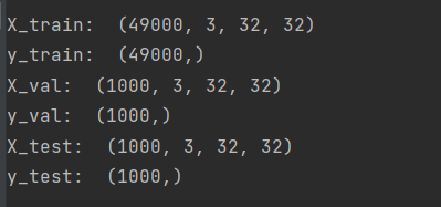
data = get_CIFAR10_data()
for k, v in data.items():
  print('%s: ' % k, v.shape)

在这里插入图片描述

卷积网络的核心是卷积运算。在cs231n/layers.py文件中，在函数conv_forward_naive中实现卷积层的前向传递。
在这一点上你不需要太担心效率;只要以您认为最清楚的方式编写代码即可。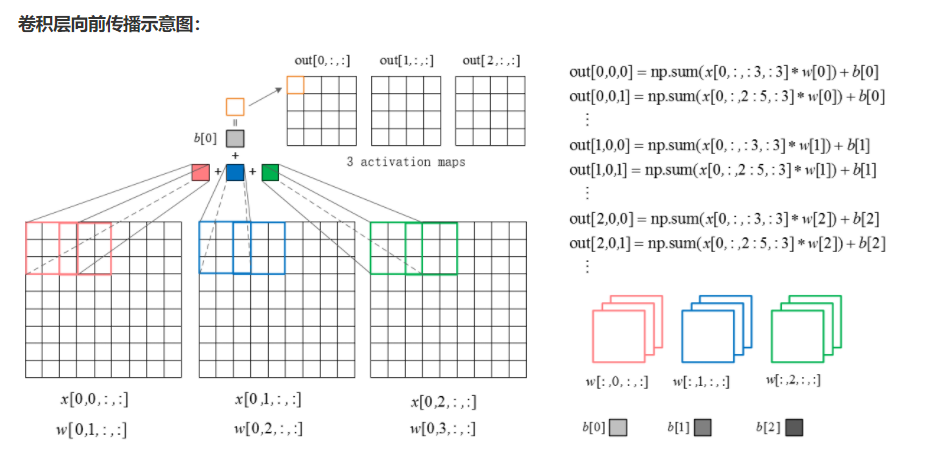在这里插入图片描述

def conv_forward_naive(x, w, b, conv_param):
    """
    A naive implementation of the forward pass for a convolutional layer.

    The input consists of N data points, each with C channels, height H and
    width W. We convolve each input with F different filters, where each filter
    spans all C channels and has height HH and width WW.

    Input:
    - x: Input data of shape (N, C, H, W)
    - w: Filter weights of shape (F, C, HH, WW)
    - b: Biases, of shape (F,)
    - conv_param: A dictionary with the following keys:
      - 'stride': The number of pixels between adjacent receptive fields in the
        horizontal and vertical directions.
      - 'pad': The number of pixels that will be used to zero-pad the input. 
        

    During padding, 'pad' zeros should be placed symmetrically (i.e equally on both sides)
    along the height and width axes of the input. Be careful not to modfiy the original
    input x directly.

    Returns a tuple of:
    - out: Output data, of shape (N, F, H', W') where H' and W' are given by
      H' = 1 + (H + 2 * pad - HH) / stride
      W' = 1 + (W + 2 * pad - WW) / stride
    - cache: (x, w, b, conv_param)
    """
    out = None
    ###########################################################################
    # TODO: Implement the convolutional forward pass.                         #
    # Hint: you can use the function np.pad for padding.                      #
    ###########################################################################
    pad = conv_param['pad']
    stride = conv_param['stride']
    N, C, H, W = x.shape
    F, C, FH, FW = w.shape

    assert (H - FH + 2 * pad) % stride == 0
    assert (W - FW + 2 * pad) % stride == 0
    outH = 1 + (H - FH + 2 * pad) // stride
    outW = 1 + (W - FW + 2 * pad) // stride

    # create output tensor after convolution layer
    out = np.zeros((N, F, outH, outW))

    # padding all input data
    x_pad = np.pad(x, ((0,0), (0,0),(pad,pad),(pad,pad)), 'constant')
    H_pad, W_pad = x_pad.shape[2], x_pad.shape[3]    

    # create w_row matrix
    w_row = w.reshape(F, C*FH*FW)                            #[F x C*FH*FW]

    # create x_col matrix with values that each neuron is connected to
    x_col = np.zeros((C*FH*FW, outH*outW))                   #[C*FH*FW x H'*W']
    for index in range(N):
        neuron = 0 
        for i in range(0, H_pad-FH+1, stride):
            for j in range(0, W_pad-FW+1,stride):
                x_col[:,neuron] = x_pad[index,:,i:i+FH,j:j+FW].reshape(C*FH*FW)
                neuron += 1
        out[index] = (w_row.dot(x_col) + b.reshape(F,1)).reshape(F, outH, outW)
    ###########################################################################
    #                             END OF YOUR CODE                            #
    ###########################################################################
    cache = (x_pad, w, b, conv_param)
    return out, cache

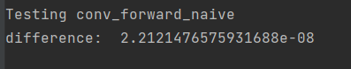
你可以通过运行以下程序来测试你的实现:
ln[3]:

x_shape = (2, 3, 4, 4)
w_shape = (3, 3, 4, 4)
x = np.linspace(-0.1, 0.5, num=np.prod(x_shape)).reshape(x_shape)
w = np.linspace(-0.2, 0.3, num=np.prod(w_shape)).reshape(w_shape)
b = np.linspace(-0.1, 0.2, num=3)

conv_param = {'stride': 2, 'pad': 1}
out, _ = conv_forward_naive(x, w, b, conv_param)
correct_out = np.array([[[[-0.08759809, -0.10987781],
                           [-0.18387192, -0.2109216 ]],
                          [[ 0.21027089,  0.21661097],
                           [ 0.22847626,  0.23004637]],
                          [[ 0.50813986,  0.54309974],
                           [ 0.64082444,  0.67101435]]],
                         [[[-0.98053589, -1.03143541],
                           [-1.19128892, -1.24695841]],
                          [[ 0.69108355,  0.66880383],
                           [ 0.59480972,  0.56776003]],
                          [[ 2.36270298,  2.36904306],
                           [ 2.38090835,  2.38247847]]]])

# Compare your output to ours; difference should be around e-8
print('Testing conv_forward_naive')
print('difference: ', rel_error(out, correct_out))

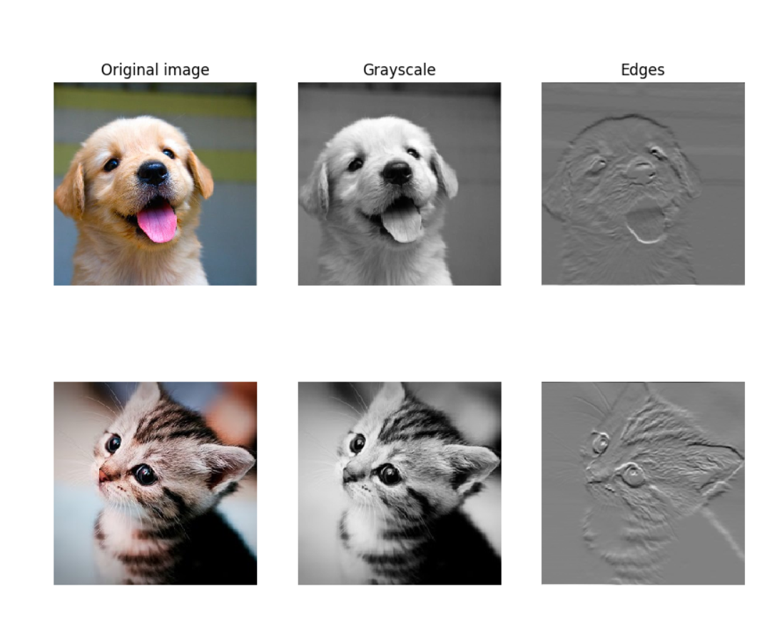
通过卷积进行图像处理

作为一种有趣的方法，既可以检查你的实现，也可以更好地理解卷积层可以执行的操作类型，我们将设置一个包含两个图像的输入，并手动设置过滤器，执行常见的图像处理操作(灰度转换和边缘检测)。卷积前向传递将对每个输入图像应用这些操作。然后我们可以将结果可视化为完整性检查。
ln[4]:

from imageio import imread
from PIL import Image

kitten = imread('cs231n/notebook_images/kitten.jpg')
puppy = imread('cs231n/notebook_images/puppy.jpg')
# kitten is wide, and puppy is already square
d = kitten.shape[1] - kitten.shape[0]
kitten_cropped = kitten[:, d//2:-d//2, :]

img_size = 200   # Make this smaller if it runs too slow
resized_puppy = np.array(Image.fromarray(puppy).resize((img_size, img_size)))
resized_kitten = np.array(Image.fromarray(kitten_cropped).resize((img_size, img_size)))
x = np.zeros((2, 3, img_size, img_size))
x[0, :, :, :] = resized_puppy.transpose((2, 0, 1))
x[1, :, :, :] = resized_kitten.transpose((2, 0, 1))

# Set up a convolutional weights holding 2 filters, each 3x3
w = np.zeros((2, 3, 3, 3))

# The first filter converts the image to grayscale.
# Set up the red, green, and blue channels of the filter.
w[0, 0, :, :] = [[0, 0, 0], [0, 0.3, 0], [0, 0, 0]]
w[0, 1, :, :] = [[0, 0, 0], [0, 0.6, 0], [0, 0, 0]]
w[0, 2, :, :] = [[0, 0, 0], [0, 0.1, 0], [0, 0, 0]]

# Second filter detects horizontal edges in the blue channel.
w[1, 2, :, :] = [[1, 2, 1], [0, 0, 0], [-1, -2, -1]]

# Vector of biases. We don't need any bias for the grayscale
# filter, but for the edge detection filter we want to add 128
# to each output so that nothing is negative.
b = np.array([0, 128])

# Compute the result of convolving each input in x with each filter in w,
# offsetting by b, and storing the results in out.
out, _ = conv_forward_naive(x, w, b, {'stride': 1, 'pad': 1})

def imshow_no_ax(img, normalize=True):
    """ Tiny helper to show images as uint8 and remove axis labels """
    if normalize:
        img_max, img_min = np.max(img), np.min(img)
        img = 255.0 * (img - img_min) / (img_max - img_min)
    plt.imshow(img.astype('uint8'))
    plt.gca().axis('off')

# Show the original images and the results of the conv operation
plt.subplot(2, 3, 1)
imshow_no_ax(puppy, normalize=False)
plt.title('Original image')
plt.subplot(2, 3, 2)
imshow_no_ax(out[0, 0])
plt.title('Grayscale')
plt.subplot(2, 3, 3)
imshow_no_ax(out[0, 1])
plt.title('Edges')
plt.subplot(2, 3, 4)
imshow_no_ax(kitten_cropped, normalize=False)
plt.subplot(2, 3, 5)
imshow_no_ax(out[1, 0])
plt.subplot(2, 3, 6)
imshow_no_ax(out[1, 1])
plt.show()

在cs231n/layers.py文件中的函数conv_backward_naive中实现卷积操作的向后传递。同样，你不需要太担心计算效率。

def conv_backward_naive(dout, cache):
    """
    A naive implementation of the backward pass for a convolutional layer.

    Inputs:
    - dout: Upstream derivatives.
    - cache: A tuple of (x, w, b, conv_param) as in conv_forward_naive

    Returns a tuple of:
    - dx: Gradient with respect to x
    - dw: Gradient with respect to w
    - db: Gradient with respect to b
    """
    dx, dw, db = None, None, None
    ###########################################################################
    # TODO: Implement the convolutional backward pass.                        #
    ###########################################################################
    x_pad, w, b, conv_param = cache
    N, F, outH, outW = dout.shape
    N, C, Hpad, Wpad = x_pad.shape
    FH, FW = w.shape[2], w.shape[3]
    stride = conv_param['stride']
    pad = conv_param['pad']

    # initialize gradients
    dx = np.zeros((N, C, Hpad - 2*pad, Wpad - 2*pad))
    dw, db = np.zeros(w.shape), np.zeros(b.shape)

    # create w_row matrix
    w_row = w.reshape(F, C*FH*FW)                            #[F x C*FH*FW]

    # create x_col matrix with values that each neuron is connected to
    x_col = np.zeros((C*FH*FW, outH*outW))                   #[C*FH*FW x H'*W']
    for index in range(N):
        out_col = dout[index].reshape(F, outH*outW)          #[F x H'*W']
        w_out = w_row.T.dot(out_col)                         #[C*FH*FW x H'*W']
        dx_cur = np.zeros((C, Hpad, Wpad))
        neuron = 0
        for i in range(0, Hpad-FH+1, stride):
            for j in range(0, Wpad-FW+1, stride):
                dx_cur[:,i:i+FH,j:j+FW] += w_out[:,neuron].reshape(C,FH,FW)
                x_col[:,neuron] = x_pad[index,:,i:i+FH,j:j+FW].reshape(C*FH*FW)
                neuron += 1
        dx[index] = dx_cur[:,pad:-pad, pad:-pad]
        dw += out_col.dot(x_col.T).reshape(F,C,FH,FW)
        db += out_col.sum(axis=1)
    ###########################################################################
    #                             END OF YOUR CODE                            #
    ###########################################################################
    return dx, dw, db

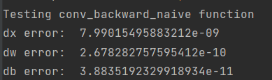
当你完成后，运行下面的检查你的向后通过一个数字梯度检查。
In[5]:

np.random.seed(231)
x = np.random.randn(4, 3, 5, 5)
w = np.random.randn(2, 3, 3, 3)
b = np.random.randn(2,)
dout = np.random.randn(4, 2, 5, 5)
conv_param = {'stride': 1, 'pad': 1}

dx_num = eval_numerical_gradient_array(lambda x: conv_forward_naive(x, w, b, conv_param)[0], x, dout)
dw_num = eval_numerical_gradient_array(lambda w: conv_forward_naive(x, w, b, conv_param)[0], w, dout)
db_num = eval_numerical_gradient_array(lambda b: conv_forward_naive(x, w, b, conv_param)[0], b, dout)

out, cache = conv_forward_naive(x, w, b, conv_param)
dx, dw, db = conv_backward_naive(dout, cache)

# Your errors should be around e-8 or less.
print('Testing conv_backward_naive function')
print('dx error: ', rel_error(dx, dx_num))
print('dw error: ', rel_error(dw, dw_num))
print('db error: ', rel_error(db, db_num))

Max-Pooling

在文件cs231n/layers.py中的函数max_pool_forward_naive中实现max-pooling操作的forward传递

def max_pool_forward_naive(x, pool_param):
    """
    A naive implementation of the forward pass for a max-pooling layer.

    Inputs:
    - x: Input data, of shape (N, C, H, W)
    - pool_param: dictionary with the following keys:
      - 'pool_height': The height of each pooling region
      - 'pool_width': The width of each pooling region
      - 'stride': The distance between adjacent pooling regions

    No padding is necessary here. Output size is given by 

    Returns a tuple of:
    - out: Output data, of shape (N, C, H', W') where H' and W' are given by
      H' = 1 + (H - pool_height) / stride
      W' = 1 + (W - pool_width) / stride
    - cache: (x, pool_param)
    """
    out = None
    ###########################################################################
    # TODO: Implement the max-pooling forward pass                            #
    ###########################################################################
    N, C, H, W = x.shape
    stride = pool_param['stride']
    PH = pool_param['pool_height']
    PW = pool_param['pool_width']
    outH = 1 + (H - PH) // stride
    outW = 1 + (W - PW) // stride

    # create output tensor for pooling layer
    out = np.zeros((N, C, outH, outW))
    for index in range(N):
        out_col = np.zeros((C, outH*outW))
        neuron = 0
        for i in range(0, H - PH + 1, stride):
            for j in range(0, W - PW + 1, stride):
                pool_region = x[index,:,i:i+PH,j:j+PW].reshape(C,PH*PW)
                out_col[:,neuron] = pool_region.max(axis=1)
                neuron += 1
        out[index] = out_col.reshape(C, outH, outW)
    ###########################################################################
    #                             END OF YOUR CODE                            #
    ###########################################################################
    cache = (x, pool_param)
    return out, cache

Test forward pass:
ln[6]:

x_shape = (2, 3, 4, 4)
x = np.linspace(-0.3, 0.4, num=np.prod(x_shape)).reshape(x_shape)
pool_param = {'pool_width': 2, 'pool_height': 2, 'stride': 2}

out, _ = max_pool_forward_naive(x, pool_param)

correct_out = np.array([[[[-0.26315789, -0.24842105],
                          [-0.20421053, -0.18947368]],
                         [[-0.14526316, -0.13052632],
                          [-0.08631579, -0.07157895]],
                         [[-0.02736842, -0.01263158],
                          [ 0.03157895,  0.04631579]]],
                        [[[ 0.09052632,  0.10526316],
                          [ 0.14947368,  0.16421053]],
                         [[ 0.20842105,  0.22315789],
                          [ 0.26736842,  0.28210526]],
                         [[ 0.32631579,  0.34105263],
                          [ 0.38526316,  0.4       ]]]])

# Compare your output with ours. Difference should be on the order of e-8.
print('Testing max_pool_forward_naive function:')
print('difference: ', rel_error(out, correct_out))

在文件cs231n/layers.py中的函数max_pool_backward_naive中实现max-pooling操作的backward传递

def max_pool_backward_naive(dout, cache):
    """
    A naive implementation of the backward pass for a max-pooling layer.

    Inputs:
    - dout: Upstream derivatives
    - cache: A tuple of (x, pool_param) as in the forward pass.

    Returns:
    - dx: Gradient with respect to x
    """
    dx = None
    ###########################################################################
    # TODO: Implement the max-pooling backward pass                           #
    ###########################################################################
    x, pool_param = cache
    N, C, outH, outW = dout.shape
    H, W = x.shape[2], x.shape[3]
    stride = pool_param['stride']
    PH, PW = pool_param['pool_height'], pool_param['pool_width']

    # initialize gradient
    dx = np.zeros(x.shape)
    
    for index in range(N):
        dout_row = dout[index].reshape(C, outH*outW)
        neuron = 0
        for i in range(0, H-PH+1, stride):
            for j in range(0, W-PW+1, stride):
                pool_region = x[index,:,i:i+PH,j:j+PW].reshape(C,PH*PW)
                max_pool_indices = pool_region.argmax(axis=1)
                dout_cur = dout_row[:,neuron]
                neuron += 1
                # pass gradient only through indices of max pool
                dmax_pool = np.zeros(pool_region.shape)
                dmax_pool[np.arange(C),max_pool_indices] = dout_cur
                dx[index,:,i:i+PH,j:j+PW] += dmax_pool.reshape(C,PH,PW)
    ###########################################################################
    #                             END OF YOUR CODE                            #
    ###########################################################################
    return dx

ln[7]:

np.random.seed(231)
x = np.random.randn(3, 2, 8, 8)
dout = np.random.randn(3, 2, 4, 4)
pool_param = {'pool_height': 2, 'pool_width': 2, 'stride': 2}

dx_num = eval_numerical_gradient_array(lambda x: max_pool_forward_naive(x, pool_param)[0], x, dout)

out, cache = max_pool_forward_naive(x, pool_param)
dx = max_pool_backward_naive(dout, cache)

# Your error should be on the order of e-12
print('Testing max_pool_backward_naive function:')
print('dx error: ', rel_error(dx, dx_num))

快速层

使卷积和池化层快速是很有挑战性的。为了避免麻烦，我们在cs231n/fast_layers.py文件中提供了卷积和池层的前向和后向传递的快速实现。

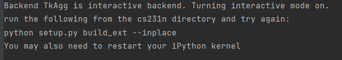
快速卷积实现依赖于Cython扩展;要编译它，你需要从cs231n目录运行以下命令:

Python setup.py build_ext——inplace

卷积层和池层的快速版本的API与上面实现的朴素版本完全相同:前向传递接收数据、权重和参数，并产生输出和缓存对象;反向传递接收上游的导数和缓存对象，并产生相对于数据和权重的梯度。

注意:只有当池区域不重叠和平铺输入时，池的快速实现才会执行得最优。如果不满足这些条件，那么快速池的实现将不会比单纯的实现快很多。

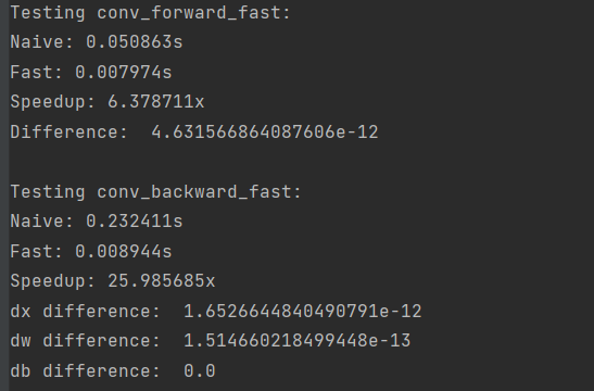
你可以通过运行以下程序来比较这些层的简单版本和快速版本的性能:
ln[8]:

# Rel errors should be around e-9 or less
from cs231n.fast_layers import conv_forward_fast, conv_backward_fast
from time import time
np.random.seed(231)
x = np.random.randn(100, 3, 31, 31)
w = np.random.randn(25, 3, 3, 3)
b = np.random.randn(25,)
dout = np.random.randn(100, 25, 16, 16)
conv_param = {'stride': 2, 'pad': 1}

t0 = time()
out_naive, cache_naive = conv_forward_naive(x, w, b, conv_param)
t1 = time()
out_fast, cache_fast = conv_forward_fast(x, w, b, conv_param)
t2 = time()

print('Testing conv_forward_fast:')
print('Naive: %fs' % (t1 - t0))
print('Fast: %fs' % (t2 - t1))
print('Speedup: %fx' % ((t1 - t0) / (t2 - t1)))
print('Difference: ', rel_error(out_naive, out_fast))

t0 = time()
dx_naive, dw_naive, db_naive = conv_backward_naive(dout, cache_naive)
t1 = time()
dx_fast, dw_fast, db_fast = conv_backward_fast(dout, cache_fast)
t2 = time()

print('\nTesting conv_backward_fast:')
print('Naive: %fs' % (t1 - t0))
print('Fast: %fs' % (t2 - t1))
print('Speedup: %fx' % ((t1 - t0) / (t2 - t1)))
print('dx difference: ', rel_error(dx_naive, dx_fast))
print('dw difference: ', rel_error(dw_naive, dw_fast))
print('db difference: ', rel_error(db_naive, db_fast))

在这里插入图片描述

ln[9]:

# Relative errors should be close to 0.0
from cs231n.fast_layers import max_pool_forward_fast, max_pool_backward_fast
np.random.seed(231)
x = np.random.randn(100, 3, 32, 32)
dout = np.random.randn(100, 3, 16, 16)
pool_param = {'pool_height': 2, 'pool_width': 2, 'stride': 2}

t0 = time()
out_naive, cache_naive = max_pool_forward_naive(x, pool_param)
t1 = time()
out_fast, cache_fast = max_pool_forward_fast(x, pool_param)
t2 = time()

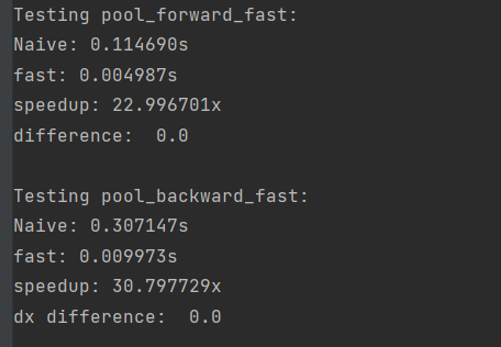
print('Testing pool_forward_fast:')
print('Naive: %fs' % (t1 - t0))
print('fast: %fs' % (t2 - t1))
print('speedup: %fx' % ((t1 - t0) / (t2 - t1)))
print('difference: ', rel_error(out_naive, out_fast))

t0 = time()
dx_naive = max_pool_backward_naive(dout, cache_naive)
t1 = time()
dx_fast = max_pool_backward_fast(dout, cache_fast)
t2 = time()

print('\nTesting pool_backward_fast:')
print('Naive: %fs' % (t1 - t0))
print('fast: %fs' % (t2 - t1))
print('speedup: %fx' % ((t1 - t0) / (t2 - t1)))
print('dx difference: ', rel_error(dx_naive, dx_fast))

“三明治”层

前面我们介绍了“三明治”层的概念，它将多个操作组合成常用的模式。在文件cs231n/layer_utils.py中，您将发现实现了一些用于卷积网络的常用模式的三明治层。
ln[10]:

from cs231n.layer_utils import conv_relu_pool_forward, conv_relu_pool_backward
np.random.seed(231)
x = np.random.randn(2, 3, 16, 16)
w = np.random.randn(3, 3, 3, 3)
b = np.random.randn(3,)
dout = np.random.randn(2, 3, 8, 8)
conv_param = {'stride': 1, 'pad': 1}
pool_param = {'pool_height': 2, 'pool_width': 2, 'stride': 2}

out, cache = conv_relu_pool_forward(x, w, b, conv_param, pool_param)
dx, dw, db = conv_relu_pool_backward(dout, cache)

dx_num = eval_numerical_gradient_array(lambda x: conv_relu_pool_forward(x, w, b, conv_param, pool_param)[0], x, dout)
dw_num = eval_numerical_gradient_array(lambda w: conv_relu_pool_forward(x, w, b, conv_param, pool_param)[0], w, dout)
db_num = eval_numerical_gradient_array(lambda b: conv_relu_pool_forward(x, w, b, conv_param, pool_param)[0], b, dout)

# Relative errors should be around e-8 or less
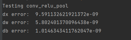
print('Testing conv_relu_pool')
print('dx error: ', rel_error(dx_num, dx))
print('dw error: ', rel_error(dw_num, dw))
print('db error: ', rel_error(db_num, db))

在这里插入图片描述
ln[11]:

from cs231n.layer_utils import conv_relu_forward, conv_relu_backward
np.random.seed(231)
x = np.random.randn(2, 3, 8, 8)
w = np.random.randn(3, 3, 3, 3)
b = np.random.randn(3,)
dout = np.random.randn(2, 3, 8, 8)
conv_param = {'stride': 1, 'pad': 1}

out, cache = conv_relu_forward(x, w, b, conv_param)
dx, dw, db = conv_relu_backward(dout, cache)

dx_num = eval_numerical_gradient_array(lambda x: conv_relu_forward(x, w, b, conv_param)[0], x, dout)
dw_num = eval_numerical_gradient_array(lambda w: conv_relu_forward(x, w, b, conv_param)[0], w, dout)
db_num = eval_numerical_gradient_array(lambda b: conv_relu_forward(x, w, b, conv_param)[0], b, dout)

# Relative errors should be around e-8 or less
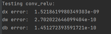
print('Testing conv_relu:')
print('dx error: ', rel_error(dx_num, dx))
print('dw error: ', rel_error(dw_num, dw))
print('db error: ', rel_error(db_num, db))

三层卷积网络

现在你已经实现了所有必要的层，我们可以把它们放在一起组成一个简单的卷积网络。

打开文件cs231n/classifier /cnn.py，完成ThreeLayerConvNet类的实现。记住你可以在你的实现中使用快速/三明治层(已经为你导入了)。

class ThreeLayerConvNet(object):
    """
    A three-layer convolutional network with the following architecture:

    conv - relu - 2x2 max pool - affine - relu - affine - softmax

    The network operates on minibatches of data that have shape (N, C, H, W)
    consisting of N images, each with height H and width W and with C input
    channels.
    """

    def __init__(self, input_dim=(3, 32, 32), num_filters=32, filter_size=7,
                 hidden_dim=100, num_classes=10, weight_scale=1e-3, reg=0.0,
                 dtype=np.float32):
        """
        Initialize a new network.

        Inputs:
        - input_dim: Tuple (C, H, W) giving size of input data
        - num_filters: Number of filters to use in the convolutional layer
        - filter_size: Width/height of filters to use in the convolutional layer
        - hidden_dim: Number of units to use in the fully-connected hidden layer
        - num_classes: Number of scores to produce from the final affine layer.
        - weight_scale: Scalar giving standard deviation for random initialization
          of weights.
        - reg: Scalar giving L2 regularization strength
        - dtype: numpy datatype to use for computation.
        """
        self.params = {}
        self.reg = reg
        self.dtype = dtype

        ############################################################################
        # TODO: Initialize weights and biases for the three-layer convolutional    #
        # network. Weights should be initialized from a Gaussian centered at 0.0   #
        # with standard deviation equal to weight_scale; biases should be          #
        # initialized to zero. All weights and biases should be stored in the      #
        #  dictionary self.params. Store weights and biases for the convolutional  #
        # layer using the keys 'W1' and 'b1'; use keys 'W2' and 'b2' for the       #
        # weights and biases of the hidden affine layer, and keys 'W3' and 'b3'    #
        # for the weights and biases of the output affine layer.                   #
        #                                                                          #
        # IMPORTANT: For this assignment, you can assume that the padding          #
        # and stride of the first convolutional layer are chosen so that           #
        # **the width and height of the input are preserved**. Take a look at      #
        # the start of the loss() function to see how that happens.                #                           
        ############################################################################
        C, H, W = input_dim
        HP, WP = 1 + (H - 2)//2, 1 + (W - 2)//2  # max pooling
        self.params['W1'] = weight_scale * np.random.randn(num_filters, C, filter_size, filter_size)
        self.params['b1'] = np.zeros(num_filters)
        self.params['W2'] = weight_scale * np.random.randn(num_filters*HP*WP, hidden_dim)
        self.params['b2'] = np.zeros(hidden_dim)
        self.params['W3'] = weight_scale * np.random.randn(hidden_dim, num_classes)
        self.params['b3'] = np.zeros(num_classes)
        ############################################################################
        #                             END OF YOUR CODE                             #
        ############################################################################

        for k, v in self.params.items():
            self.params[k] = v.astype(dtype)


    def loss(self, X, y=None):
        """
        Evaluate loss and gradient for the three-layer convolutional network.

        Input / output: Same API as TwoLayerNet in fc_net.py.
        """
        W1, b1 = self.params['W1'], self.params['b1']
        W2, b2 = self.params['W2'], self.params['b2']
        W3, b3 = self.params['W3'], self.params['b3']

        # pass conv_param to the forward pass for the convolutional layer
        # Padding and stride chosen to preserve the input spatial size
        filter_size = W1.shape[2]
        conv_param = {'stride': 1, 'pad': (filter_size - 1) // 2}

        # pass pool_param to the forward pass for the max-pooling layer
        pool_param = {'pool_height': 2, 'pool_width': 2, 'stride': 2}

        scores = None
        ############################################################################
        # TODO: Implement the forward pass for the three-layer convolutional net,  #
        # computing the class scores for X and storing them in the scores          #
        # variable.                                                                #
        #                                                                          #
        # Remember you can use the functions defined in cs231n/fast_layers.py and  #
        # cs231n/layer_utils.py in your implementation (already imported).         #
        ############################################################################
        pool_out, cache = conv_relu_pool_forward(X, W1, b1, conv_param, pool_param)
        X2, fc_cache = affine_relu_forward(pool_out, W2, b2)
        scores, fc2_cache = affine_forward(X2, W3, b3)
        ############################################################################
        #                             END OF YOUR CODE                             #
        ############################################################################

        if y is None:
            return scores

        loss, grads = 0, {}
        ############################################################################
        # TODO: Implement the backward pass for the three-layer convolutional net, #
        # storing the loss and gradients in the loss and grads variables. Compute  #
        # data loss using softmax, and make sure that grads[k] holds the gradients #
        # for self.params[k]. Don't forget to add L2 regularization!               #
        #                                                                          #
        # NOTE: To ensure that your implementation matches ours and you pass the   #
        # automated tests, make sure that your L2 regularization includes a factor #
        # of 0.5 to simplify the expression for the gradient.                      #
        ############################################################################
        loss, softmax_grad = softmax_loss(scores, y)
        loss += 0.5 * self.reg * np.sum(W1 * W1)
        loss += 0.5 * self.reg * np.sum(W2 * W2)
        loss += 0.5 * self.reg * np.sum(W3 * W3)
        
        # backpropagation of gradients
        dout, grads['W3'], grads['b3'] = affine_backward(softmax_grad, fc2_cache)
        dout, grads['W2'], grads['b2'] = affine_relu_backward(dout, fc_cache)
        dout, grads['W1'], grads['b1'] = conv_relu_pool_backward(dout, cache)
        
        # L2 regularization
        grads['W1'] += self.reg * W1
        grads['W2'] += self.reg * W2
        grads['W3'] += self.reg * W3
        ############################################################################
        #                             END OF YOUR CODE                             #
        ############################################################################

        return loss, grads

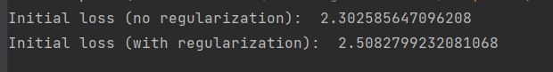
检查损失

在您建立一个新的网络之后，您应该做的第一件事是检查损失。当我们使用softmax损失时，我们预计随机权值(和无正则化)的损失是关于C类的log©。当我们加入正规化时，这个会增加。
ln[12]:

model = ThreeLayerConvNet()

N = 50
X = np.random.randn(N, 3, 32, 32)
y = np.random.randint(10, size=N)

loss, grads = model.loss(X, y)
print('Initial loss (no regularization): ', loss)

model.reg = 0.5
loss, grads = model.loss(X, y)
print('Initial loss (with regularization): ', loss)

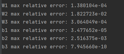
梯度检查

在损失看起来合理之后，使用数值梯度检查以确保向后传递是正确的。当你使用数值梯度检查时，你应该在每层使用少量的人工数据和少量的神经元。注意:正确的实现可能仍然存在e-2级的相对错误。
ln[13]:

num_inputs = 2
input_dim = (3, 16, 16)
reg = 0.0
num_classes = 10
np.random.seed(231)
X = np.random.randn(num_inputs, *input_dim)
y = np.random.randint(num_classes, size=num_inputs)

model = ThreeLayerConvNet(num_filters=3, filter_size=3,
                          input_dim=input_dim, hidden_dim=7,
                          dtype=np.float64)
loss, grads = model.loss(X, y)
# Errors should be small, but correct implementations may have
# relative errors up to the order of e-2
for param_name in sorted(grads):
    f = lambda _: model.loss(X, y)[0]
    param_grad_num = eval_numerical_gradient(f, model.params[param_name], verbose=False, h=1e-6)
    e = rel_error(param_grad_num, grads[param_name])
    print('%s max relative error: %e' % (param_name, rel_error(param_grad_num, grads[param_name])))

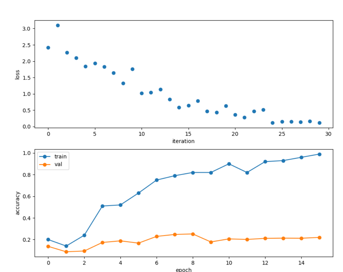
过拟合小的数据集
一个很好的技巧是用几个训练样本来训练您的模型。您应该能够过拟合小数据集，这将导致非常高的训练精度和相对较低的验证精度。
ln[14]:

np.random.seed(231)

num_train = 100
small_data = {
  'X_train': data['X_train'][:num_train],
  'y_train': data['y_train'][:num_train],
  'X_val': data['X_val'],
  'y_val': data['y_val'],
}

model = ThreeLayerConvNet(weight_scale=1e-2)

solver = Solver(model, small_data,
                num_epochs=15, batch_size=50,
                update_rule='adam',
                optim_config={
                  'learning_rate': 1e-3,
                },
                verbose=True, print_every=1)
solver.train()

(Iteration 1 / 30) loss: 2.414060
(Epoch 0 / 15) train acc: 0.200000; val_acc: 0.137000
(Iteration 2 / 30) loss: 3.102925
(Epoch 1 / 15) train acc: 0.140000; val_acc: 0.087000
(Iteration 3 / 30) loss: 2.270330
(Iteration 4 / 30) loss: 2.096705
(Epoch 2 / 15) train acc: 0.240000; val_acc: 0.094000
(Iteration 5 / 30) loss: 1.838880
(Iteration 6 / 30) loss: 1.934188
(Epoch 3 / 15) train acc: 0.510000; val_acc: 0.173000
(Iteration 7 / 30) loss: 1.827912
(Iteration 8 / 30) loss: 1.639574
(Epoch 4 / 15) train acc: 0.520000; val_acc: 0.188000
(Iteration 9 / 30) loss: 1.330082
(Iteration 10 / 30) loss: 1.756115
(Epoch 5 / 15) train acc: 0.630000; val_acc: 0.167000
(Iteration 11 / 30) loss: 1.024162
(Iteration 12 / 30) loss: 1.041826
(Epoch 6 / 15) train acc: 0.750000; val_acc: 0.229000
(Iteration 13 / 30) loss: 1.142777
(Iteration 14 / 30) loss: 0.835706
(Epoch 7 / 15) train acc: 0.790000; val_acc: 0.247000
(Iteration 15 / 30) loss: 0.587786
(Iteration 16 / 30) loss: 0.645509
(Epoch 8 / 15) train acc: 0.820000; val_acc: 0.252000
(Iteration 17 / 30) loss: 0.786844
(Iteration 18 / 30) loss: 0.467054
(Epoch 9 / 15) train acc: 0.820000; val_acc: 0.178000
(Iteration 19 / 30) loss: 0.429880
(Iteration 20 / 30) loss: 0.635498
(Epoch 10 / 15) train acc: 0.900000; val_acc: 0.206000
(Iteration 21 / 30) loss: 0.365807
(Iteration 22 / 30) loss: 0.284220
(Epoch 11 / 15) train acc: 0.820000; val_acc: 0.201000
(Iteration 23 / 30) loss: 0.469343
(Iteration 24 / 30) loss: 0.509369
(Epoch 12 / 15) train acc: 0.920000; val_acc: 0.211000
(Iteration 25 / 30) loss: 0.111638
(Iteration 26 / 30) loss: 0.145388
(Epoch 13 / 15) train acc: 0.930000; val_acc: 0.213000
(Iteration 27 / 30) loss: 0.155575
(Iteration 28 / 30) loss: 0.143398
(Epoch 14 / 15) train acc: 0.960000; val_acc: 0.212000
(Iteration 29 / 30) loss: 0.158160
(Iteration 30 / 30) loss: 0.118934
(Epoch 15 / 15) train acc: 0.990000; val_acc: 0.220000
绘制损失、训练准确性和验证准确性应显示清楚的过拟合:
ln[15]:

plt.subplot(2, 1, 1)
plt.plot(solver.loss_history, 'o')
plt.xlabel('iteration')
plt.ylabel('loss')

plt.subplot(2, 1, 2)
plt.plot(solver.train_acc_history, '-o')
plt.plot(solver.val_acc_history, '-o')
plt.legend(['train', 'val'], loc='upper left')
plt.xlabel('epoch')
plt.ylabel('accuracy')
plt.show()

在这里插入图片描述
通过对三层卷积网络进行一次训练，在训练集上的准确率应该大于40%:
ln[16]:

model = ThreeLayerConvNet(weight_scale=0.001, hidden_dim=500, reg=0.001)

solver = Solver(model, data,
                num_epochs=1, batch_size=50,
                update_rule='adam',
                optim_config={
                  'learning_rate': 1e-3,
                },
                verbose=True, print_every=20)
solver.train()

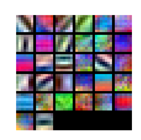
可视化的过滤器

你可以通过运行以下程序来可视化训练网络的第一层卷积过滤器:
ln[17]:

from cs231n.vis_utils import visualize_grid

grid = visualize_grid(model.params['W1'].transpose(0, 2, 3, 1))
plt.imshow(grid.astype('uint8'))
plt.axis('off')
plt.gcf().set_size_inches(5, 5)
plt.show()

空间批正常化

我们已经看到，批处理标准化是训练深度全连接网络的一种非常有用的技术。正如原论文Sergey Ioffe and Christian Szegedy, “Batch Normalization: Accelerating Deep Network Training by Reducing Internal Covariate Shift”, ICML 2015.中提出的，批处理标准化也可以用于卷积网络，但我们需要对其进行一点调整;这个修改将被称为“空间批处理标准化”。

通常batch-normalization接受输入的形状(N, D)和产生输出的形状(N, D),我们整个minibatch标准化维度数据来自卷积N层,批规范化需要接受输入的形状(N,C, H, W)和产生输出的形状(N, C, H,W)，其中N维给出了迷你批大小，(H, W)维给出了特征图的空间大小。

如果feature map是使用卷积生成的，那么我们期望每个feature channel的统计量在不同图像之间以及同一图像内不同位置之间都是相对一致的。因此，空间批处理标准化通过计算最小批处理维数N和空间维数H和W的统计量来计算每个C特征通道的平均值和方差。

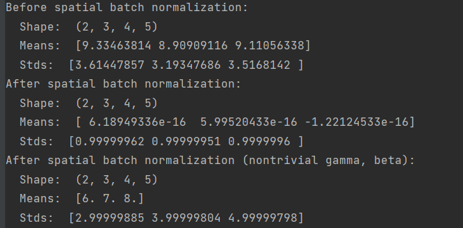
空间批处理标准化:forward pass

在文件cs231n/layers.py中，在函数spatial_batchnorm_forward中实现空间批处理标准化的前向传递。运行以下命令检查您的实现:

def spatial_batchnorm_forward(x, gamma, beta, bn_param):
    """
    Computes the forward pass for spatial batch normalization.

    Inputs:
    - x: Input data of shape (N, C, H, W)
    - gamma: Scale parameter, of shape (C,)
    - beta: Shift parameter, of shape (C,)
    - bn_param: Dictionary with the following keys:
      - mode: 'train' or 'test'; required
      - eps: Constant for numeric stability
      - momentum: Constant for running mean / variance. momentum=0 means that
        old information is discarded completely at every time step, while
        momentum=1 means that new information is never incorporated. The
        default of momentum=0.9 should work well in most situations.
      - running_mean: Array of shape (D,) giving running mean of features
      - running_var Array of shape (D,) giving running variance of features

    Returns a tuple of:
    - out: Output data, of shape (N, C, H, W)
    - cache: Values needed for the backward pass
    """
    out, cache = None, None

    ###########################################################################
    # TODO: Implement the forward pass for spatial batch normalization.       #
    #                                                                         #
    # HINT: You can implement spatial batch normalization by calling the      #
    # vanilla version of batch normalization you implemented above.           #
    # Your implementation should be very short; ours is less than five lines. #
    ###########################################################################
    N, C, H, W = x.shape
    x = x.transpose(0,2,3,1).reshape(N*H*W, C)
    out, cache = batchnorm_forward(x, gamma, beta, bn_param)
    out = out.reshape(N, H, W, C).transpose(0,3,1,2)
    ###########################################################################
    #                             END OF YOUR CODE                            #
    ###########################################################################

    return out, cache

ln[18]:

np.random.seed(231)
# Check the training-time forward pass by checking means and variances
# of features both before and after spatial batch normalization

N, C, H, W = 2, 3, 4, 5
x = 4 * np.random.randn(N, C, H, W) + 10

print('Before spatial batch normalization:')
print('  Shape: ', x.shape)
print('  Means: ', x.mean(axis=(0, 2, 3)))
print('  Stds: ', x.std(axis=(0, 2, 3)))

# Means should be close to zero and stds close to one
gamma, beta = np.ones(C), np.zeros(C)
bn_param = {'mode': 'train'}
out, _ = spatial_batchnorm_forward(x, gamma, beta, bn_param)
print('After spatial batch normalization:')
print('  Shape: ', out.shape)
print('  Means: ', out.mean(axis=(0, 2, 3)))
print('  Stds: ', out.std(axis=(0, 2, 3)))

# Means should be close to beta and stds close to gamma
gamma, beta = np.asarray([3, 4, 5]), np.asarray([6, 7, 8])
out, _ = spatial_batchnorm_forward(x, gamma, beta, bn_param)
print('After spatial batch normalization (nontrivial gamma, beta):')
print('  Shape: ', out.shape)
print('  Means: ', out.mean(axis=(0, 2, 3)))
print('  Stds: ', out.std(axis=(0, 2, 3)))

ln[19]:

np.random.seed(231)
# Check the test-time forward pass by running the training-time
# forward pass many times to warm up the running averages, and then
# checking the means and variances of activations after a test-time
# forward pass.
N, C, H, W = 10, 4, 11, 12

bn_param = {'mode': 'train'}
gamma = np.ones(C)
beta = np.zeros(C)
for t in range(50):
  x = 2.3 * np.random.randn(N, C, H, W) + 13
  spatial_batchnorm_forward(x, gamma, beta, bn_param)
bn_param['mode'] = 'test'
x = 2.3 * np.random.randn(N, C, H, W) + 13
a_norm, _ = spatial_batchnorm_forward(x, gamma, beta, bn_param)

# Means should be close to zero and stds close to one, but will be
# noisier than training-time forward passes.
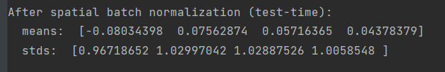
print('After spatial batch normalization (test-time):')
print('  means: ', a_norm.mean(axis=(0, 2, 3)))
print('  stds: ', a_norm.std(axis=(0, 2, 3)))

反向传递：

def spatial_batchnorm_backward(dout, cache):
    """
    Computes the backward pass for spatial batch normalization.

    Inputs:
    - dout: Upstream derivatives, of shape (N, C, H, W)
    - cache: Values from the forward pass

    Returns a tuple of:
    - dx: Gradient with respect to inputs, of shape (N, C, H, W)
    - dgamma: Gradient with respect to scale parameter, of shape (C,)
    - dbeta: Gradient with respect to shift parameter, of shape (C,)
    """
    dx, dgamma, dbeta = None, None, None

    ###########################################################################
    # TODO: Implement the backward pass for spatial batch normalization.      #
    #                                                                         #
    # HINT: You can implement spatial batch normalization by calling the      #
    # vanilla version of batch normalization you implemented above.           #
    # Your implementation should be very short; ours is less than five lines. #
    ###########################################################################
    N, C, H, W = dout.shape
    dout = dout.transpose(0,2,3,1).reshape(N*H*W, C)
    dx, dgamma, dbeta = batchnorm_backward_alt(dout, cache)
    dx = dx.reshape(N, H, W, C).transpose(0,3,1,2)
    ###########################################################################
    #                             END OF YOUR CODE                            #
    ###########################################################################

    return dx, dgamma, dbeta

ln[20]:

np.random.seed(231)
N, C, H, W = 2, 3, 4, 5
x = 5 * np.random.randn(N, C, H, W) + 12
gamma = np.random.randn(C)
beta = np.random.randn(C)
dout = np.random.randn(N, C, H, W)

bn_param = {'mode': 'train'}
fx = lambda x: spatial_batchnorm_forward(x, gamma, beta, bn_param)[0]
fg = lambda a: spatial_batchnorm_forward(x, gamma, beta, bn_param)[0]
fb = lambda b: spatial_batchnorm_forward(x, gamma, beta, bn_param)[0]

dx_num = eval_numerical_gradient_array(fx, x, dout)
da_num = eval_numerical_gradient_array(fg, gamma, dout)
db_num = eval_numerical_gradient_array(fb, beta, dout)

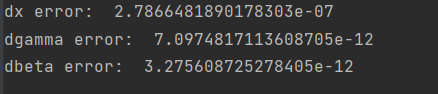
#You should expect errors of magnitudes between 1e-12~1e-06
_, cache = spatial_batchnorm_forward(x, gamma, beta, bn_param)
dx, dgamma, dbeta = spatial_batchnorm_backward(dout, cache)
print('dx error: ', rel_error(dx_num, dx))
print('dgamma error: ', rel_error(da_num, dgamma))
print('dbeta error: ', rel_error(db_num, dbeta))

Group Normalization:

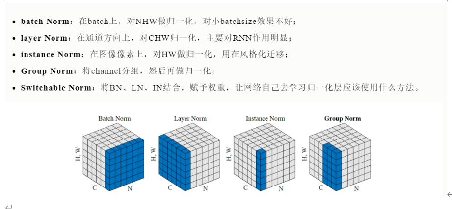
在之前的作业中，我们提到过Layer Normalization是一种替代的标准化技术，它减轻了batch Normalization的批大小限制。然而当使用卷积层时，层标准化的性能不如批处理标准化:

在完全连接的层中，层中的所有隐藏单元都倾向于对最终预测做出类似的贡献，重新定位和重新缩放对层的求和输入效果很好。然而，类似贡献的假设不再适用于卷积神经网络。接收域位于图像边界附近的大量隐藏单元很少被打开，因此与同一层内的其他隐藏单元的统计数据有很大的不同。

提出了一种中间技术。与Layer Normalization(对每个数据点的整个特性进行标准化)相反，他们建议将每个数据点特性一致地拆分为组，然后进行每组每数据点的标准化。

在文件cs231n/layers.py中，在函数spatial_groupnorm_forward中实现组标准化的前向传递。

def spatial_groupnorm_forward(x, gamma, beta, G, gn_param):
    """
    Computes the forward pass for spatial group normalization.
    In contrast to layer normalization, group normalization splits each entry 
    in the data into G contiguous pieces, which it then normalizes independently.
    Per feature shifting and scaling are then applied to the data, in a manner identical to that of batch normalization and layer normalization.

    Inputs:
    - x: Input data of shape (N, C, H, W)
    - gamma: Scale parameter, of shape (C,)
    - beta: Shift parameter, of shape (C,)
    - G: Integer mumber of groups to split into, should be a divisor of C
    - gn_param: Dictionary with the following keys:
      - eps: Constant for numeric stability

    Returns a tuple of:
    - out: Output data, of shape (N, C, H, W)
    - cache: Values needed for the backward pass
    """
    out, cache = None, None
    eps = gn_param.get('eps',1e-5)
    ###########################################################################
    # TODO: Implement the forward pass for spatial group normalization.       #
    # This will be extremely similar to the layer norm implementation.        #
    # In particular, think about how you could transform the matrix so that   #
    # the bulk of the code is similar to both train-time batch normalization  #
    # and layer normalization!                                                # 
    ###########################################################################
    N, C, H, W = x.shape
    size = (N*G, C//G *H*W)
    x = x.reshape(size).T
    gamma = gamma.reshape(1, C, 1, 1)
    beta = beta.reshape(1, C, 1, 1)
    # similar to batch normalization
    mu = x.mean(axis=0)
    var = x.var(axis=0) + eps
    std = np.sqrt(var)
    z = (x - mu)/std
    z = z.T.reshape(N, C, H, W)
    out = gamma * z + beta
    # save values for backward call
    cache={'std':std, 'gamma':gamma, 'z':z, 'size':size}
    ###########################################################################
    #                             END OF YOUR CODE                            #
    ###########################################################################
    return out, cache

运行以下命令检查您的实现:
ln[21]:

np.random.seed(231)
# Check the training-time forward pass by checking means and variances
# of features both before and after spatial batch normalization

N, C, H, W = 2, 6, 4, 5
G = 2
x = 4 * np.random.randn(N, C, H, W) + 10
x_g = x.reshape((N*G,-1))
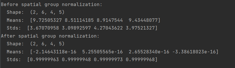
print('Before spatial group normalization:')
print('  Shape: ', x.shape)
print('  Means: ', x_g.mean(axis=1))
print('  Stds: ', x_g.std(axis=1))

# Means should be close to zero and stds close to one
gamma, beta = np.ones((1,C,1,1)), np.zeros((1,C,1,1))
bn_param = {'mode': 'train'}

out, _ = spatial_groupnorm_forward(x, gamma, beta, G, bn_param)
out_g = out.reshape((N*G,-1))
print('After spatial group normalization:')
print('  Shape: ', out.shape)
print('  Means: ', out_g.mean(axis=1))
print('  Stds: ', out_g.std(axis=1))

backward pass:

def spatial_groupnorm_backward(dout, cache):
    """
    Computes the backward pass for spatial group normalization.

    Inputs:
    - dout: Upstream derivatives, of shape (N, C, H, W)
    - cache: Values from the forward pass

    Returns a tuple of:
    - dx: Gradient with respect to inputs, of shape (N, C, H, W)
    - dgamma: Gradient with respect to scale parameter, of shape (C,)
    - dbeta: Gradient with respect to shift parameter, of shape (C,)
    """
    dx, dgamma, dbeta = None, None, None

    ###########################################################################
    # TODO: Implement the backward pass for spatial group normalization.      #
    # This will be extremely similar to the layer norm implementation.        #
    ###########################################################################
    N, C, H, W = dout.shape
    size = cache['size']
    dbeta = dout.sum(axis=(0,2,3), keepdims=True)
    dgamma = np.sum(dout * cache['z'], axis=(0,2,3), keepdims=True)

    # reshape tensors
    z = cache['z'].reshape(size).T
    M = z.shape[0]
    dfdz = dout * cache['gamma']
    dfdz = dfdz.reshape(size).T
    # copy from batch normalization backward alt
    dfdz_sum = np.sum(dfdz,axis=0)
    dx = dfdz - dfdz_sum/M - np.sum(dfdz * z,axis=0) * z/M
    dx /= cache['std']
    dx = dx.T.reshape(N, C, H, W)
    ###########################################################################
    #                             END OF YOUR CODE                            #
    ###########################################################################
    return dx, dgamma, dbeta

ln[22]:

np.random.seed(231)
N, C, H, W = 2, 6, 4, 5
G = 2
x = 5 * np.random.randn(N, C, H, W) + 12
gamma = np.random.randn(1,C,1,1)
beta = np.random.randn(1,C,1,1)
dout = np.random.randn(N, C, H, W)

gn_param = {}
fx = lambda x: spatial_groupnorm_forward(x, gamma, beta, G, gn_param)[0]
fg = lambda a: spatial_groupnorm_forward(x, gamma, beta, G, gn_param)[0]
fb = lambda b: spatial_groupnorm_forward(x, gamma, beta, G, gn_param)[0]

dx_num = eval_numerical_gradient_array(fx, x, dout)
da_num = eval_numerical_gradient_array(fg, gamma, dout)
db_num = eval_numerical_gradient_array(fb, beta, dout)

_, cache = spatial_groupnorm_forward(x, gamma, beta, G, gn_param)
dx, dgamma, dbeta = spatial_groupnorm_backward(dout, cache)

#You should expect errors of magnitudes between 1e-12~1e-07
print('dx error: ', rel_error(dx_num, dx))
print('dgamma error: ', rel_error(da_num, dgamma))
print('dbeta error: ', rel_error(db_num, dbeta))

Esaka7

关注

4
点赞
踩
12

收藏

觉得还不错? 一键收藏
打赏
1
评论
CS231n-assignment2-Convolutional Networks

卷积网络到目前为止，我们已经使用了深度全连接网络，使用它们探索不同的优化策略和网络架构。全连接网络是一个很好的实验平台，因为它们的计算效率非常高，但实际上所有最先进的结果都使用卷积网络。首先，您将实现在卷积网络中使用的几种层类型。然后，您将使用这些层来训练CIFAR-10数据集上的卷积网络。ln[1]:# As usual, a bit of setupimport numpy as npimport matplotlib.pyplot as pltfrom cs231n.classifier
复制链接

扫一扫