【吴恩达深度学习】01_week2_Logistic Regression with a Neural Network mindset

作业链接

Logistic Regression with a Neural Network mindset

Welcome to your first (required) programming assignment! You will build a logistic regression classifier to recognize cats. This assignment will step you through how to do this with a Neural Network mindset, and so will also hone your intuitions about deep learning.

Instructions:

• Do not use loops (for/while) in your code, unless the instructions explicitly ask you to do so.

You will learn to:

• Build the general architecture of a learning algorithm, including:
  • Initializing parameters
  • Calculating the cost function and its gradient
  • Using an optimization algorithm (gradient descent)
• Gather all three functions above into a main model function, in the right order.

具有神经网络的逻辑回归

欢迎来到你的第一个（必做）编程作业！你将用逻辑回归分类器来识别猫，这项作业将带你逐步了解如何用神经网络思维来做这件事, 并且也将磨练你深度学习的直觉。

说明:

• 在你的代码中不要使用循环(for/while)，除了明确的要求你使用。

你将学到:

• 构建学习算法的整体结构,包括:
  • 初始化参数
  • 计算损失函数和梯度
  • 使用优化算法 (梯度下降)
• 按照正确的顺序，将上述的三个函数合成一个主模块函数.

1 - Packages

First, let’s run the cell below to import all the packages that you will need during this assignment.

• numpy is the fundamental package for scientific computing with Python.
• h5py is a common package to interact with a dataset that is stored on an H5 file.
• matplotlib is a famous library to plot graphs in Python.
• PIL and scipy are used here to test your model with your own picture at the end.

1 - 包

首先, 让我们运行下面的单元来导入本次作业所需要的所有包.

• numpy 是Python用于科学计算的基本包.
• h5py 是与以H5文件形式存储的数据库进行交互的通用包.
• matplotlib 是Python著名的库用于绘制图形.
• PIL 和 scipy 是在最后用你自己的图片测试你的模型.

import numpy as np
import matplotlib.pyplot as plt
import h5py
import scipy
from PIL import Image
from scipy import ndimage
from lr_utils import load_dataset

%matplotlib inline

2 - Overview of the Problem set

Problem Statement: You are given a dataset (“data.h5”) containing:
- a training set of m_train images labeled as cat (y=1) or non-cat (y=0)
- a test set of m_test images labeled as cat or non-cat
- each image is of shape (num_px, num_px, 3) where 3 is for the 3 channels (RGB). Thus, each image is square (height = num_px) and (width = num_px).

You will build a simple image-recognition algorithm that can correctly classify pictures as cat or non-cat.

Let’s get more familiar with the dataset. Load the data by running the following code.

2 - 问题集概论

问题陈述: 你有数据库 (“data.h5”) 包含:
- m_train 个图像和标签（猫（y=1）或不是猫（y=0））的一个训练集
- m_test 个图像和标签（猫或不是猫）的一个测试集
- 每个图像的尺寸 (num_px, num_px, 3) 3表示有3个通道 (RGB). 因此, 每个图像是正方形 (height = num_px) 且 (width = num_px).

你将搭建一个简单的图像分类算法用于正确的分类图像是猫或不是猫.

让我们熟悉下数据集. 通过运行下面代码来载入数据集.

# Loading the data (cat/non-cat)
train_set_x_orig, train_set_y, test_set_x_orig, test_set_y, classes = load_dataset()

We added “_orig” at the end of image datasets (train and test) because we are going to preprocess them. After preprocessing, we will end up with train_set_x and test_set_x (the labels train_set_y and test_set_y don’t need any preprocessing).

Each line of your train_set_x_orig and test_set_x_orig is an array representing an image. You can visualize an example by running the following code. Feel free also to change the index value and re-run to see other images.

添加 “_orig” 在图像数据库末尾 (训练和测试) 是因为我们要进行预处理. 预处理之后, 我们得到 train_set_x 和 test_set_x (标签 train_set_y 和 test_set_y 不需要任何预处理).

每一行 train_set_x_orig 和 test_set_x_orig 是一个代表图像的数组. 你可以通过运行以下代码来可视化示例. 可以改变 index 值重新运行来查看其他图片

# Example of a picture
index = 10
plt.imshow(train_set_x_orig[index])
print ("y = " + str(train_set_y[:, index]) + ", it's a '" + classes[np.squeeze(train_set_y[:, index])].decode("utf-8") +  "' picture.")

Many software bugs in deep learning come from having matrix/vector dimensions that don’t fit. If you can keep your matrix/vector dimensions straight you will go a long way toward eliminating many bugs.

Exercise: Find the values for:
- m_train (number of training examples)
- m_test (number of test examples)
- num_px (= height = width of a training image)
Remember that train_set_x_orig is a numpy-array of shape (m_train, num_px, num_px, 3). For instance, you can access m_train by writing train_set_x_orig.shape[0].

深度学习中的很多bug是由于矩阵/向量维度不匹配. 如果你可以保持矩阵/向量的维度，那么你能消除很多错误.

练习: 查找以下的值:
- m_train (训练数据的个数)
- m_test (测试数据的个数)
- num_px (= 训练图像的高 = 训练图像的宽)
记住， train_set_x_orig 是一个大小为 (m_train, num_px, num_px, 3)的 numpy-array . 例如, 你可以通过 train_set_x_orig.shape[0]来获得
m_train .

### START CODE HERE ### (≈ 3 lines of code)
m_train=train_set_x_orig.shape[0]
m_test=test_set_x_orig.shape[0]
num_px=train_set_x_orig.shape[1]
### END CODE HERE ###

print ("Number of training examples: m_train = " + str(m_train))
print ("Number of testing examples: m_test = " + str(m_test))
print ("Height/Width of each image: num_px = " + str(num_px))
print ("Each image is of size: (" + str(num_px) + ", " + str(num_px) + ", 3)")
print ("train_set_x shape: " + str(train_set_x_orig.shape))
print ("train_set_y shape: " + str(train_set_y.shape))
print ("test_set_x shape: " + str(test_set_x_orig.shape))
print ("test_set_y shape: " + str(test_set_y.shape))

Expected Output for m_train, m_test and num_px:

**m_train**	209
**m_test**	50
**num_px**	64

For convenience, you should now reshape images of shape (num_px, num_px, 3) in a numpy-array of shape (num_px $\ast$ num_px $\ast$ 3, 1). After this, our training (and test) dataset is a numpy-array where each column represents a flattened image. There should be m_train (respectively m_test) columns.

Exercise: Reshape the training and test data sets so that images of size (num_px, num_px, 3) are flattened into single vectors of shape (num_px $\ast$ num_px $\ast$ 3, 1).

A trick when you want to flatten a matrix X of shape (a,b,c,d) to a matrix X_flatten of shape (b$\ast$c$\ast$d, a) is to use:

X_flatten = X.reshape(X.shape[0], -1).T      # X.T is the transpose of X

为了方便, 你现在应该将numpy-array的维度从 (num_px, num_px, 3) 变为 (num_px $\ast$ num_px $\ast$ 3, 1). 在这之后, 我们训练 (测试) 数据集是一个每列代表一个展平的图像的numpy-array . 这应该有 m_train (m_test) 列.

练习: 改变训练集和测试集的形状，将图像的尺寸 (num_px, num_px, 3) 展成单个向量 (num_px $\ast$ num_px $\ast$ 3, 1).

小技巧：当你想将矩阵 X (a,b,c,d) 展平为 X_flatten (b$\ast$c$\ast$d, a) 你可以用:

X_flatten = X.reshape(X.shape[0], -1).T      # X.T 是 X 的转置

# Reshape the training and test examples

### START CODE HERE ### (≈ 2 lines of code)
train_set_x_flatten=train_set_x_orig.reshape(train_set_x_orig.shape[0],-1).T
test_set_x_flatten=test_set_x_orig.reshape(test_set_x_orig.shape[0],-1).T
### END CODE HERE ###

print ("train_set_x_flatten shape: " + str(train_set_x_flatten.shape))
print ("train_set_y shape: " + str(train_set_y.shape))
print ("test_set_x_flatten shape: " + str(test_set_x_flatten.shape))
print ("test_set_y shape: " + str(test_set_y.shape))
print ("sanity check after reshaping: " + str(train_set_x_flatten[0:5,0]))

Expected Output:

**train_set_x_flatten shape**	(12288, 209)
**train_set_y shape**	(1, 209)
**test_set_x_flatten shape**	(12288, 50)
**test_set_y shape**	(1, 50)
**sanity check after reshaping**	[17 31 56 22 33]

To represent color images, the red, green and blue channels (RGB) must be specified for each pixel, and so the pixel value is actually a vector of three numbers ranging from 0 to 255.

One common preprocessing step in machine learning is to center and standardize your dataset, meaning that you substract the mean of the whole numpy array from each example, and then divide each example by the standard deviation of the whole numpy array. But for picture datasets, it is simpler and more convenient and works almost as well to just divide every row of the dataset by 255 (the maximum value of a pixel channel).

During the training of your model, you’re going to multiply weights and add biases to some initial inputs in order to observe neuron activations. Then you backpropogate with the gradients to train the model. But, it is extremely important for each feature to have a similar range such that our gradients don’t explode. You will see that more in detail later in the lectures. !

Let’s standardize our dataset.

为了表示彩色图像, 并须为每个像素指明红, 绿，蓝三个通道 (RGB),实际上像素的值是三个0到255数字的向量.

机器学习中常见的预处理是中心化和标准化数据集,意思是 numpy 数组中的每个元素都要减去数组的平均值,再除以整个数组的标准差. 但是对于图片数据集,只需要每一列除以255 (像素通道的最大值)，这很简单、方便而且效果差不多.

在训练你模型的过程中, 为了观察神经元的激活，你需要对初始输入乘以权重和加上偏置值.然后反向传播用梯度训练模型. 但是, 让每个特征都有一个相似的范围，这样梯度就不会爆炸，这一点非常重要. 具体细节你将在后续课程中见到. !

让我们标准化数据集.

train_set_x = train_set_x_flatten/255.
test_set_x = test_set_x_flatten/255.

What you need to remember:

Common steps for pre-processing a new dataset are:

• Figure out the dimensions and shapes of the problem (m_train, m_test, num_px, …)
• Reshape the datasets such that each example is now a vector of size (num_px * num_px * 3, 1)
• “Standardize” the data

你应该记住:

预处理一个新的数据集的常见步骤为:

• 找出问题的维度和形状(m_train, m_test, num_px, …)
• 重塑数据集的形状，使每个样本的大小为一个 (num_px * num_px * 3, 1)的向量
• “标准化” 数据

3 - General Architecture of the learning algorithm

It’s time to design a simple algorithm to distinguish cat images from non-cat images.

You will build a Logistic Regression, using a Neural Network mindset. The following Figure explains why Logistic Regression is actually a very simple Neural Network!

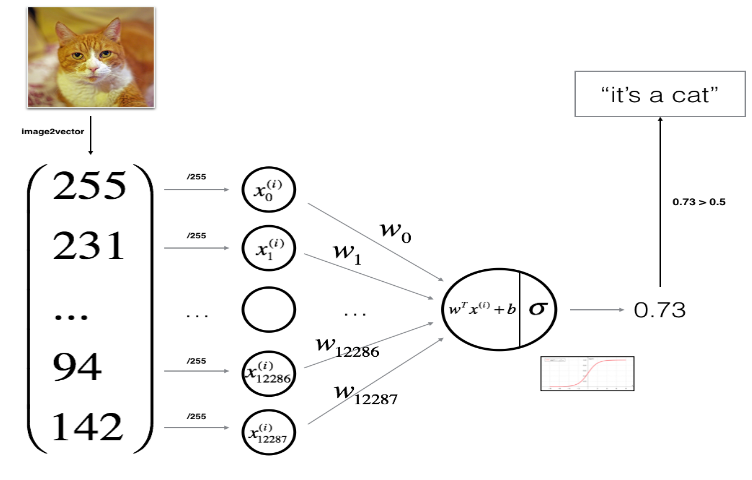
Mathematical expression of the algorithm:

For one example $x^{(i)}$:
$$z^{(i)}=w^T{x}^{(i)}+b\text{\hspace{1em}(1)}$$
$${\hat{y}}^{(i)}=a^{(i)}=sigmoid(z^{(i)})\text{\hspace{1em}(2)}$$
$$\mathcal{L}(a^{(i)},y^{(i)})=-y^{(i)}\log (a^{(i)})-(1-y^{(i)})\log (1-a^{(i)})\text{\hspace{1em}(3)}$$

The cost is then computed by summing over all training examples:
$$J=\frac{1}{m}\sum _{i=1}^m\mathcal{L}(a^{(i)},y^{(i)})\text{\hspace{1em}(6)}$$

Key steps:
In this exercise, you will carry out the following steps:
- Initialize the parameters of the model
- Learn the parameters for the model by minimizing the cost
- Use the learned parameters to make predictions (on the test set)
- Analyse the results and conclude

3 - 学习算法的一般框架

是时候设计一个简单算法用于区分猫图和非猫图.

你将使用神经网络创建一个逻辑回归. 下面说明了为什么 逻辑回归事实上是一个很简单的神经网络!

算法的数学表示:

对于样本 $x^{(i)}$:
$$z^{(i)}=w^T{x}^{(i)}+b\text{\hspace{1em}(1)}$$
$${\hat{y}}^{(i)}=a^{(i)}=sigmoid(z^{(i)})\text{\hspace{1em}(2)}$$
$$\mathcal{L}(a^{(i)},y^{(i)})=-y^{(i)}\log (a^{(i)})-(1-y^{(i)})\log (1-a^{(i)})\text{\hspace{1em}(3)}$$

通过所有样本的求和来计算损失:
$$J=\frac{1}{m}\sum _{i=1}^m\mathcal{L}(a^{(i)},y^{(i)})\text{\hspace{1em}(6)}$$

关键步骤:
在本次练习中, 你讲执行以下步骤:
- 初始化模型的参数
- 学习模型的参数以最小化损失
- 使用学习到的参数进行预测 (在测试集上)
- 分析结果并得出结论

4 - Building the parts of our algorithm

The main steps for building a Neural Network are:

1. Define the model structure (such as number of input features)
2. Initialize the model’s parameters
3. Loop:
   • Calculate current loss (forward propagation)
   • Calculate current gradient (backward propagation)
   • Update parameters (gradient descent)

You often build 1-3 separately and integrate them into one function we call model().

4.1 - Helper functions

Exercise: Using your code from “Python Basics”, implement sigmoid(). As you’ve seen in the figure above, you need to compute $sigmoid(w^{T}x+b)=\frac{1}{1+e^{-(w^{T}x+b)}}$ to make predictions. Use np.exp().

4 -构建算法的各个部分

构建神经网络的主要步骤是:

1. 定义模型的结构 (例如输入特征的数量)
2. 初始化模型的参数
3. 循环:
   • 计算当前损失 (前向传播)
   • 计算当前梯度 (反向传播)
   • 更新参数 (梯度下降)

你通常分别构建 1-3 并整合到一个函数 model().

4.1 - 辅助函数

练习: 使用 "Python Basics"中的代码, 实现 sigmoid()，上图所示, 你需要计算 $sigmoid(w^{T}x+b)=\frac{1}{1+e^{-(w^{T}x+b)}}$ 进行预测. 使用 np.exp().

# GRADED FUNCTION: sigmoid

def sigmoid(z):
    """
    Compute the sigmoid of z

    Arguments:
    z -- A scalar or numpy array of any size.

    Return:
    s -- sigmoid(z)
    """

    ### START CODE HERE ### (≈ 1 line of code)
    s=1/(1+np.exp(-z))
    ### END CODE HERE ###
    
    return s

print ("sigmoid([0, 2]) = " + str(sigmoid(np.array([0,2]))))

Expected Output:

**sigmoid([0, 2])**

[ 0.5 0.88079708]

4.2 - Initializing parameters

Exercise: Implement parameter initialization in the cell below. You have to initialize w as a vector of zeros. If you don’t know what numpy function to use, look up np.zeros() in the Numpy library’s documentation.

4.2 - 初始化参数

练习: 在下面的单元中实现参数初始化. 你必须将w初始化为一个零向量.如果你不知道如何使用numpy函数, 在 Numpy 库文档中查阅 np.zeros().

# GRADED FUNCTION: initialize_with_zeros

def initialize_with_zeros(dim):
    """
    This function creates a vector of zeros of shape (dim, 1) for w and initializes b to 0.
    
    Argument:
    dim -- size of the w vector we want (or number of parameters in this case)
    
    Returns:
    w -- initialized vector of shape (dim, 1)
    b -- initialized scalar (corresponds to the bias)
    """
    
    ### START CODE HERE ### (≈ 1 line of code)
    w,b=np.zeros((dim,1)),0
    ### END CODE HERE ###

    assert(w.shape == (dim, 1))
    assert(isinstance(b, float) or isinstance(b, int))
    
    return w, b

dim = 2
w, b = initialize_with_zeros(dim)
print ("w = " + str(w))
print ("b = " + str(b))

Expected Output:

** w **	[[ 0.] [ 0.]]
** b **	0

For image inputs, w will be of shape (num_px $\times$ num_px $\times$ 3, 1).

4.3 - Forward and Backward propagation

Now that your parameters are initialized, you can do the “forward” and “backward” propagation steps for learning the parameters.

Exercise: Implement a function propagate() that computes the cost function and its gradient.

Hints:

Forward Propagation:

• You get X
• You compute $A=\sigma (w^{T}X+b)=(a^{(0)},a^{(1)},...,a^{(m-1)},a^{(m)})$
• You calculate the cost function: $J=-\frac{1}{m}{\sum }_{i=1}^m{y}^{(i)}\log (a^{(i)})+(1-y^{(i)})\log (1-a^{(i)})$

Here are the two formulas you will be using:

$$\frac{\partial J}{\partial w}=\frac{1}{m}X(A-Y{)}^T\text{\hspace{1em}(7)}$$
$$\frac{\partial J}{\partial b}=\frac{1}{m}\sum _{i=1}^m(a^{(i)}-y^{(i)})\text{\hspace{1em}(8)}$$

4.3 - 前向传播和反向传播

现在你的参数已经初始化了, 你可以做 “前向” 和 “反向” 传播步骤来学习参数.

练习: 实现函数 propagate() 计算损失函数和梯度.

Hints:

前向传播:

• 得到 X
• 计算 $A=\sigma (w^{T}X+b)=(a^{(0)},a^{(1)},...,a^{(m-1)},a^{(m)})$
• 计算损失函数: $J=-\frac{1}{m}{\sum }_{i=1}^m{y}^{(i)}\log (a^{(i)})+(1-y^{(i)})\log (1-a^{(i)})$

你将用到这两个公式:

$$\frac{\partial J}{\partial w}=\frac{1}{m}X(A-Y{)}^T\text{\hspace{1em}(7)}$$
$$\frac{\partial J}{\partial b}=\frac{1}{m}\sum _{i=1}^m(a^{(i)}-y^{(i)})\text{\hspace{1em}(8)}$$

# GRADED FUNCTION: propagate

def propagate(w, b, X, Y):
    """
    Implement the cost function and its gradient for the propagation explained above

    Arguments:
    w -- weights, a numpy array of size (num_px * num_px * 3, 1)
    b -- bias, a scalar
    X -- data of size (num_px * num_px * 3, number of examples)
    Y -- true "label" vector (containing 0 if non-cat, 1 if cat) of size (1, number of examples)

    Return:
    cost -- negative log-likelihood cost for logistic regression
    dw -- gradient of the loss with respect to w, thus same shape as w
    db -- gradient of the loss with respect to b, thus same shape as b
    
    Tips:
    - Write your code step by step for the propagation. np.log(), np.dot()
    """
    
    m = X.shape[1]
    
    # FORWARD PROPAGATION (FROM X TO COST)
    ### START CODE HERE ### (≈ 2 lines of code)
    A=sigmoid(w.T@X+b)
    cost=-np.mean(Y*np.log(A)+(1-Y)*np.log(1-A))
    ### END CODE HERE ###
    
    # BACKWARD PROPAGATION (TO FIND GRAD)
    ### START CODE HERE ### (≈ 2 lines of code)
    dw=(X@(A-Y).T)/m
    db=np.mean(A-Y)
    ### END CODE HERE ###
    assert(dw.shape == w.shape)
    assert(db.dtype == float)
    cost = np.squeeze(cost)
    assert(cost.shape == ())
    
    grads = {"dw": dw,
             "db": db}
    
    return grads, cost

w, b, X, Y = np.array([[1],[2]]), 2, np.array([[1,2],[3,4]]), np.array([[1,0]])
grads, cost = propagate(w, b, X, Y)
print ("dw = " + str(grads["dw"]))
print ("db = " + str(grads["db"]))
print ("cost = " + str(cost))

Expected Output:

** dw **	[[ 0.99993216] [ 1.99980262]]
** db **	0.499935230625
** cost **	6.000064773192205

d) Optimization

• You have initialized your parameters.
• You are also able to compute a cost function and its gradient.
• Now, you want to update the parameters using gradient descent.

Exercise: Write down the optimization function. The goal is to learn $w$ and $b$ by minimizing the cost function $J$. For a parameter $\theta$, the update rule is $ \theta = \theta - \alpha \text{ } d\theta$, where $\alpha$ is the learning rate.

d) 优化

• 初始化参数.
• 计算损失函数和梯度.
• 使用梯度下降更新参数.

练习: 编写优化函数. 目标是学习 $w$ 和 $b$ 以最小化损失函数 $J$. 对于参数 $\theta$, 更新规则是 $\theta =\theta -\alpha d\theta$, 其中$\alpha$ 是学习率.

# GRADED FUNCTION: optimize

def optimize(w, b, X, Y, num_iterations, learning_rate, print_cost = False):
    """
    This function optimizes w and b by running a gradient descent algorithm
    
    Arguments:
    w -- weights, a numpy array of size (num_px * num_px * 3, 1)
    b -- bias, a scalar
    X -- data of shape (num_px * num_px * 3, number of examples)
    Y -- true "label" vector (containing 0 if non-cat, 1 if cat), of shape (1, number of examples)
    num_iterations -- number of iterations of the optimization loop
    learning_rate -- learning rate of the gradient descent update rule
    print_cost -- True to print the loss every 100 steps
    
    Returns:
    params -- dictionary containing the weights w and bias b
    grads -- dictionary containing the gradients of the weights and bias with respect to the cost function
    costs -- list of all the costs computed during the optimization, this will be used to plot the learning curve.
    
    Tips:
    You basically need to write down two steps and iterate through them:
        1) Calculate the cost and the gradient for the current parameters. Use propagate().
        2) Update the parameters using gradient descent rule for w and b.
    """
    
    costs = []
    
    for i in range(num_iterations):
        
        
        # Cost and gradient calculation (≈ 1-4 lines of code)
        ### START CODE HERE ### 
        grads,cost=propagate(w,b,X,Y)
        ### END CODE HERE ###
        
        # Retrieve derivatives from grads
        dw = grads["dw"]
        db = grads["db"]
        
        # update rule (≈ 2 lines of code)
        ### START CODE HERE ###
        w=w-learning_rate*dw
        b=b-learning_rate*db
        ### END CODE HERE ###
        
        # Record the costs
        if i % 100 == 0:
            costs.append(cost)
        
        # Print the cost every 100 training examples
        if print_cost and i % 100 == 0:
            print ("Cost after iteration %i: %f" %(i, cost))
    
    params = {"w": w,
              "b": b}
    
    grads = {"dw": dw,
             "db": db}
    
    return params, grads, costs

params, grads, costs = optimize(w, b, X, Y, num_iterations= 100, learning_rate = 0.009, print_cost = False)

print ("w = " + str(params["w"]))
print ("b = " + str(params["b"]))
print ("dw = " + str(grads["dw"]))
print ("db = " + str(grads["db"]))
print(costs)

Expected Output:

**w**	[[ 0.1124579 ] [ 0.23106775]]
**b**	1.55930492484
**dw**	[[ 0.90158428] [ 1.76250842]]
**db**	0.430462071679

**Exercise:** The previous function will output the learned w and b. We are able to use w and b to predict the labels for a dataset X. Implement the `predict()` function. There is two steps to computing predictions:

1. Calculate $\hat{Y}=A=\sigma (w^{T}X+b)$

2. Convert the entries of a into 0 (if activation <= 0.5) or 1 (if activation > 0.5), stores the predictions in a vector Y_prediction. If you wish, you can use an if/else statement in a for loop (though there is also a way to vectorize this).

练习: 前面的函数将输出学习过的 w 和 b. 我们可以使用 w 和 b 来预测数据集 X 的标签. 实现 predict() 函数. 计算预测有两个步骤:

1. 计算 $\hat{Y}=A=\sigma (w^{T}X+b)$

2. 转换 a 为 0 (如果 a <= 0.5) 或 1 (如果 a > 0.5), 保存预测结果在 Y_prediction向量中, 你可以用 if/else 语句在for 循环中 (尽管也有一种方法可以将其向量化).

# GRADED FUNCTION: predict

def predict(w, b, X):
    '''
    Predict whether the label is 0 or 1 using learned logistic regression parameters (w, b)
    
    Arguments:
    w -- weights, a numpy array of size (num_px * num_px * 3, 1)
    b -- bias, a scalar
    X -- data of size (num_px * num_px * 3, number of examples)
    
    Returns:
    Y_prediction -- a numpy array (vector) containing all predictions (0/1) for the examples in X
    '''
    
    m = X.shape[1]
    Y_prediction = np.zeros((1,m))
    w = w.reshape(X.shape[0], 1)
    
    # Compute vector "A" predicting the probabilities of a cat being present in the picture
    ### START CODE HERE ### (≈ 1 line of code)
    A=sigmoid(w.T@X+b)
    ### END CODE HERE ###

    for i in range(A.shape[1]):
        
        # Convert probabilities A[0,i] to actual predictions p[0,i]
        ### START CODE HERE ### (≈ 4 lines of code)
        if A[0,i]<=0.5:
            Y_prediction[0,i]=0
        else:
            Y_prediction[0,i]=1
        ### END CODE HERE ###
    
    assert(Y_prediction.shape == (1, m))
    
    return Y_prediction

print ("predictions = " + str(predict(w, b, X)))

Expected Output:

**predictions**

[[ 1. 1.]]

What to remember:
You’ve implemented several functions that:

• Initialize (w,b)
• Optimize the loss iteratively to learn parameters (w,b):
  • computing the cost and its gradient
  • updating the parameters using gradient descent
• Use the learned (w,b) to predict the labels for a given set of examples

记住:
你已经实现了以下函数:

• 初始化 (w,b)
• 通过迭代来优化损失以学习参数 (w,b):
  • 计算损失和梯度
  • 用梯度下降更新参数
• 用学习好的 (w,b) 来预测给定数据集的标签

5 - Merge all functions into a model

You will now see how the overall model is structured by putting together all the building blocks (functions implemented in the previous parts) together, in the right order.

Exercise: Implement the model function. Use the following notation:
- Y_prediction_test for your predictions on the test set
- Y_prediction_train for your predictions on the train set
- w, costs, grads for the outputs of optimize()

5 - 合并所有函数为一个模型

将所有部分 (上部分实现的函数)以正确的顺序合并.

联系: 实现model函数. 使用以下命名:
- Y_prediction_test 测试集的预测
- Y_prediction_train 训练集的预测
- w, costs, grads 为 optimize()的输出

# GRADED FUNCTION: model

def model(X_train, Y_train, X_test, Y_test, num_iterations = 2000, learning_rate = 0.5, print_cost = False):
    """
    Builds the logistic regression model by calling the function you've implemented previously
    
    Arguments:
    X_train -- training set represented by a numpy array of shape (num_px * num_px * 3, m_train)
    Y_train -- training labels represented by a numpy array (vector) of shape (1, m_train)
    X_test -- test set represented by a numpy array of shape (num_px * num_px * 3, m_test)
    Y_test -- test labels represented by a numpy array (vector) of shape (1, m_test)
    num_iterations -- hyperparameter representing the number of iterations to optimize the parameters
    learning_rate -- hyperparameter representing the learning rate used in the update rule of optimize()
    print_cost -- Set to true to print the cost every 100 iterations
    
    Returns:
    d -- dictionary containing information about the model.
    """
    
    ### START CODE HERE ###
    
    # initialize parameters with zeros (≈ 1 line of code)
    w,b=initialize_with_zeros(X_train.shape[0])
    
    # Gradient descent (≈ 1 line of code)
    params,grads,costs=optimize(w, b, X_train, Y_train, num_iterations, learning_rate, print_cost)
    
    # Retrieve parameters w and b from dictionary "parameters"
    w=params['w']
    b=params['b']
    
    # Predict test/train set examples (≈ 2 lines of code)
    Y_prediction_test=predict(w,b,X_test)
    Y_prediction_train=predict(w,b,X_train)
    
    ### END CODE HERE ###

    # Print train/test Errors
    print("train accuracy: {} %".format(100 - np.mean(np.abs(Y_prediction_train - Y_train)) * 100))
    print("test accuracy: {} %".format(100 - np.mean(np.abs(Y_prediction_test - Y_test)) * 100))

    
    d = {"costs": costs,
         "Y_prediction_test": Y_prediction_test, 
         "Y_prediction_train" : Y_prediction_train, 
         "w" : w, 
         "b" : b,
         "learning_rate" : learning_rate,
         "num_iterations": num_iterations}
    
    return d

d = model(train_set_x, train_set_y, test_set_x, test_set_y, num_iterations = 2000, learning_rate = 0.005, print_cost = True)

Expected Output:

**Train Accuracy**	99.04306220095694 %
**Test Accuracy**	70.0 %

Comment: Training accuracy is close to 100%. This is a good sanity check: your model is working and has high enough capacity to fit the training data. Test error is 68%. It is actually not bad for this simple model, given the small dataset we used and that logistic regression is a linear classifier. But no worries, you’ll build an even better classifier next week!

Also, you see that the model is clearly overfitting the training data. Later in this specialization you will learn how to reduce overfitting, for example by using regularization. Using the code below (and changing the index variable) you can look at predictions on pictures of the test set.

评价: 训练准确度接近于 100%. 这是个很好的情况: 你的模型可以运行并且有足够大的容量来适合训练数据. 测试误差为 68%. 这实际上并不差, 因为我们使用的数据集比较小并且逻辑回归是一个线性分类. 但是不要担心,你在下周将搭建一个更好的分类器!

显然，模型对于训练数据明显的过拟合了. 后续你会专门的学习如何减小过拟合, 例如使用正则化.使用以下代码 (改变 index 值) 你可以查看测试集上的图片的预测

# Example of a picture that was wrongly classified.
index = 1
plt.imshow(test_set_x[:,index].reshape((num_px, num_px, 3)))
print ("y = " + str(test_set_y[0,index]) + ", you predicted that it is a \"" + classes[int(d["Y_prediction_test"][0,index])].decode("utf-8") +  "\" picture.")

Let’s also plot the cost function and the gradients.
让我们画出损失函数和梯度

# Plot learning curve (with costs)
costs = np.squeeze(d['costs'])
plt.plot(costs)
plt.ylabel('cost')
plt.xlabel('iterations (per hundreds)')
plt.title("Learning rate =" + str(d["learning_rate"]))
plt.show()

Interpretation:
You can see the cost decreasing. It shows that the parameters are being learned. However, you see that you could train the model even more on the training set. Try to increase the number of iterations in the cell above and rerun the cells. You might see that the training set accuracy goes up, but the test set accuracy goes down. This is called overfitting.
说明:
你可以看见损失下降. 这表示参数正在学习. 然而, 你可以在训练集上训练更多次.试着增加上面单元中的迭代次数然后重新运行. 你会发现训练集的准确度上升了,但测试集的准确度确下降了.这叫做过拟合.

6 - Further analysis (optional/ungraded exercise)

Congratulations on building your first image classification model. Let’s analyze it further, and examine possible choices for the learning rate $\alpha$.

6 - 进一步分析 (选做)

恭喜你搭建了你第一个图像分类模型. 让我们进一步分析,如何选取学习率 $\alpha$.

Choice of learning rate

Reminder:
In order for Gradient Descent to work you must choose the learning rate wisely. The learning rate $\alpha$ determines how rapidly we update the parameters. If the learning rate is too large we may “overshoot” the optimal value. Similarly, if it is too small we will need too many iterations to converge to the best values. That’s why it is crucial to use a well-tuned learning rate.

Let’s compare the learning curve of our model with several choices of learning rates. Run the cell below. This should take about 1 minute. Feel free also to try different values than the three we have initialized the learning_rates variable to contain, and see what happens.

选取学习率

提醒:
为了梯度下降有效，你必须明智的选择学习率. 学习率 $\alpha$ 决定了更新参数的速度. 如果学习率过大， 这将会 “超过” 最优值. 类似的,如果过小，则需要更多的迭代次数才能收敛于最优值.这就是为什么选取学习率是至关重要的.

让我们比较不同学习率下的学习率曲线. 运行下面的单元.这可能需要1分钟. 试一下learning_rates以外的值, 看看会发生什么

learning_rates = [0.01, 0.001, 0.0001]
models = {}
for i in learning_rates:
    print ("learning rate is: " + str(i))
    models[str(i)] = model(train_set_x, train_set_y, test_set_x, test_set_y, num_iterations = 1500, learning_rate = i, print_cost = False)
    print ('\n' + "-------------------------------------------------------" + '\n')

for i in learning_rates:
    plt.plot(np.squeeze(models[str(i)]["costs"]), label= str(models[str(i)]["learning_rate"]))

plt.ylabel('cost')
plt.xlabel('iterations')

legend = plt.legend(loc='upper center', shadow=True)
frame = legend.get_frame()
frame.set_facecolor('0.90')
plt.show()

Interpretation:

• Different learning rates give different costs and thus different predictions results.
• If the learning rate is too large (0.01), the cost may oscillate up and down. It may even diverge (though in this example, using 0.01 still eventually ends up at a good value for the cost).
• A lower cost doesn’t mean a better model. You have to check if there is possibly overfitting. It happens when the training accuracy is a lot higher than the test accuracy.
• In deep learning, we usually recommend that you:
  • Choose the learning rate that better minimizes the cost function.
  • If your model overfits, use other techniques to reduce overfitting. (We’ll talk about this in later videos.)

说明:

• 不同的学习率会有不同的损失和不同的预测结果.
• 如果学习率太大 (0.01), 损失可能上下波动. 甚至可能会发散 (即使在本例中, 使用 0.01 最终获得了好的损失值).
• 低损失值不代表模型好. 你必须检查是否可能过拟合.当训练精确度比测试精确度高得多的时候就发生了过拟合.
• 在深度学习中,通常建议你:
  • 选择能最小化损失函数的学习率
  • 如果你的模型过拟合了, 使用其他技术来减少过拟合. (将在后面的视频中讨论.)

7 - Test with your own image (optional/ungraded exercise)

Congratulations on finishing this assignment. You can use your own image and see the output of your model. To do that:
1. Click on “File” in the upper bar of this notebook, then click “Open” to go on your Coursera Hub.
2. Add your image to this Jupyter Notebook’s directory, in the “images” folder
3. Change your image’s name in the following code
4. Run the code and check if the algorithm is right (1 = cat, 0 = non-cat)!

7 - 测试你自己的图像 (选做)

恭喜你完成了作业.你可以使用自己的图像观察模型的输出.为此 :
1. 点击 notebook上面的 “File”, 然后点击 “Open” 进入你的 Coursera Hub.
2. 把你的图像加入 Jupyter Notebook’s 目录, “images” 文件夹中
3. 在下面的代码中修改图像的名称
4. 运行代码检查算法是否正确 (1 = 猫图, 0 = 非猫图)!

## START CODE HERE ## (PUT YOUR IMAGE NAME) 

## END CODE HERE ##

# We preprocess the image to fit your algorithm.
fname = "images/" + my_image
image = np.array(ndimage.imread(fname, flatten=False))
my_image = scipy.misc.imresize(image, size=(num_px,num_px)).reshape((1, num_px*num_px*3)).T
my_predicted_image = predict(d["w"], d["b"], my_image)

plt.imshow(image)
print("y = " + str(np.squeeze(my_predicted_image)) + ", your algorithm predicts a \"" + classes[int(np.squeeze(my_predicted_image)),].decode("utf-8") +  "\" picture.")

What to remember from this assignment:

1. Preprocessing the dataset is important.
2. You implemented each function separately: initialize(), propagate(), optimize(). Then you built a model().
3. Tuning the learning rate (which is an example of a “hyperparameter”) can make a big difference to the algorithm. You will see more examples of this later in this course!

从本次作业中你需要记住:

1. 预处理数据集很重要.
2. 你分开的实现了每个函数: initialize(), propagate(), optimize(). 然后你实现了 model().
3. 调整学习率 (这是 "超参数"的例子) 可以使算法更有效. 你将在后续课程中看到更多的例子!

Finally, if you’d like, we invite you to try different things on this Notebook. Make sure you submit before trying anything. Once you submit, things you can play with include:
- Play with the learning rate and the number of iterations
- Try different initialization methods and compare the results
- Test other preprocessings (center the data, or divide each row by its standard deviation)

最后, 如果你感兴趣, 我们邀请你在 Notebook 尝试其他操作.在试之前请确保已经提交. 一旦你提交, 你可以进行如下操作:

• 改变学习率和迭代次数
• 尝试不同的初始化方法并比较产生的结果
• 测试其他预处理 (数据中心化, 或将每行除以标准差)