人工智能-作业3：例题程序复现 PyTorch版

最新推荐文章于 2024-06-16 12:32:13 发布

+51

最新推荐文章于 2024-06-16 12:32:13 发布

阅读量209

点赞数 2

分类专栏：人工智能实验文章标签： pytorch 人工智能深度学习

本文链接：https://blog.csdn.net/qq_51776413/article/details/124644188

版权

人工智能实验专栏收录该内容

6 篇文章 1 订阅

订阅专栏

1.使用pytorch复现课上例题

在这里插入图片描述

import torch

x1, x2 = torch.Tensor([0.5]), torch.Tensor([0.3])
y1, y2 = torch.Tensor([0.23]), torch.Tensor([-0.07])
print("=====输入值：x1, x2；真实输出值：y1, y2=====")
print(x1, x2, y1, y2)
w1, w2, w3, w4, w5, w6, w7, w8 = torch.Tensor([0.2]), torch.Tensor([-0.4]), torch.Tensor([0.5]), torch.Tensor(
    [0.6]), torch.Tensor([0.1]), torch.Tensor([-0.5]), torch.Tensor([-0.3]), torch.Tensor([0.8])  # 权重初始值
w1.requires_grad = True
w2.requires_grad = True
w3.requires_grad = True
w4.requires_grad = True
w5.requires_grad = True
w6.requires_grad = True
w7.requires_grad = True
w8.requires_grad = True


def sigmoid(z):
    a = 1 / (1 + torch.exp(-z))
    return a


def forward_propagate(x1, x2):
    in_h1 = w1 * x1 + w3 * x2
    out_h1 = sigmoid(in_h1)  # out_h1 = torch.sigmoid(in_h1)
    in_h2 = w2 * x1 + w4 * x2
    out_h2 = sigmoid(in_h2)  # out_h2 = torch.sigmoid(in_h2)

    in_o1 = w5 * out_h1 + w7 * out_h2
    out_o1 = sigmoid(in_o1)  # out_o1 = torch.sigmoid(in_o1)
    in_o2 = w6 * out_h1 + w8 * out_h2
    out_o2 = sigmoid(in_o2)  # out_o2 = torch.sigmoid(in_o2)

    print("正向计算：o1 ,o2")
    print(out_o1.data, out_o2.data)

    return out_o1, out_o2


def loss_fuction(x1, x2, y1, y2):  # 损失函数
    y1_pred, y2_pred = forward_propagate(x1, x2)  # 前向传播
    loss = (1 / 2) * (y1_pred - y1) ** 2 + (1 / 2) * (y2_pred - y2) ** 2  # 考虑 ： t.nn.MSELoss()
    print("损失函数（均方误差）：", loss.item())
    return loss


def update_w(w1, w2, w3, w4, w5, w6, w7, w8):
    # 步长
    step = 1
    w1.data = w1.data - step * w1.grad.data
    w2.data = w2.data - step * w2.grad.data
    w3.data = w3.data - step * w3.grad.data
    w4.data = w4.data - step * w4.grad.data
    w5.data = w5.data - step * w5.grad.data
    w6.data = w6.data - step * w6.grad.data
    w7.data = w7.data - step * w7.grad.data
    w8.data = w8.data - step * w8.grad.data
    w1.grad.data.zero_()  # 注意：将w中所有梯度清零
    w2.grad.data.zero_()
    w3.grad.data.zero_()
    w4.grad.data.zero_()
    w5.grad.data.zero_()
    w6.grad.data.zero_()
    w7.grad.data.zero_()
    w8.grad.data.zero_()
    return w1, w2, w3, w4, w5, w6, w7, w8


if __name__ == "__main__":

    print("=====更新前的权值=====")
    print(w1.data, w2.data, w3.data, w4.data, w5.data, w6.data, w7.data, w8.data)

    for i in range(1):
        print("=====第" + str(i) + "轮=====")
        L = loss_fuction(x1, x2, y1, y2)  # 前向传播，求 Loss，构建计算图
        L.backward()  # 自动求梯度，不需要人工编程实现。反向传播，求出计算图中所有梯度存入w中
        print("\tgrad W: ", round(w1.grad.item(), 2), round(w2.grad.item(), 2), round(w3.grad.item(), 2),
              round(w4.grad.item(), 2), round(w5.grad.item(), 2), round(w6.grad.item(), 2), round(w7.grad.item(), 2),
              round(w8.grad.item(), 2))
        w1, w2, w3, w4, w5, w6, w7, w8 = update_w(w1, w2, w3, w4, w5, w6, w7, w8)

    print("更新后的权值")
    print(w1.data, w2.data, w3.data, w4.data, w5.data, w6.data, w7.data, w8.data)

运行结果：

=====输入值：x1, x2；真实输出值：y1, y2=====
tensor([0.5000]) tensor([0.3000]) tensor([0.2300]) tensor([-0.0700])
=====更新前的权值=====
tensor([0.2000]) tensor([-0.4000]) tensor([0.5000]) tensor([0.6000]) tensor([0.1000]) tensor([-0.5000]) tensor([-0.3000]) tensor([0.8000])
=====第0轮=====
正向计算：o1 ,o2
tensor([0.4769]) tensor([0.5287])
损失函数（均方误差）： 0.2097097933292389
	grad W:  -0.01 0.01 -0.01 0.01 0.03 0.08 0.03 0.07
更新后的权值
tensor([0.2084]) tensor([-0.4126]) tensor([0.5051]) tensor([0.5924]) tensor([0.0654]) tensor([-0.5839]) tensor([-0.3305]) tensor([0.7262])

2.对比【作业3】和【作业2】的程序，观察两种方法结果是否相同？如果不同，哪个正确？

两种方法结果不同，作业三PyTorch版正确。

3.【作业2】程序更新

反向传播部分代码更新见“人工智能-作业2：例题程序复现”
初始权值和数据集：
在这里插入图片描述
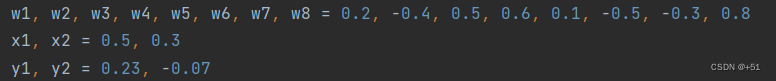
更改“step = 1”后运行一轮如下：

=====输入值：x1, x2；真实输出值：y1, y2=====
0.5 0.3 0.23 -0.07
=====更新前的权值=====
0.2 -0.4 0.5 0.6 0.1 -0.5 -0.3 0.8
=====第0轮=====
正向计算：o1 ,o2
0.47695 0.5287
损失函数：均方误差
0.20971
w的梯度: -0.00843 0.01264 -0.00506 0.00758 0.03463 0.08387 0.03049 0.07384
更新后的权值
0.21 -0.41 0.51 0.59 0.07 -0.58 -0.33 0.73

可以看到与PyTorch版本运行结果中更新后的权值结果相同。

4.对比【作业2】与【作业3】的反向传播的实现方法。总结并陈述。

作业2中的方法通过手动计算，得到反向传播过程中各参数梯度；作业3通过张量Tensor求Loss，构建计算图，在最后通过backword()自动求梯度。

5.激活函数Sigmoid用PyTorch自带函数torch.sigmoid()，观察、总结并陈述。

原本写的激活函数：
在这里插入图片描述
使用PyTorch自带的激活函数：

自带的函数具有易于求导的特性，但其计算量也更大。

6.激活函数Sigmoid改变为Relu，观察、总结并陈述。

relu函数定义为：f(x) = max(0,x)
在这里插入图片描述
线性整流作为神经元的激活函数，定义了该神经元在线性变换 $\mathbf{w}^\mathrm{T}x+b$ 之后的非线性输出结果。该函数可以加快训练速度。

7.损失函数MSE用PyTorch自带函数 t.nn.MSELoss()替代，观察、总结并陈述。

	loss_func = torch.nn.MSELoss() #自带函数
    y_pred = torch.cat((y1_pred, y2_pred), dim=0) 
    y = torch.cat((y1, y2), dim=0)  
    loss = loss_func(y_pred, y)

通过预测值和实际值y_pred和y计算函数的损失值loss。

8.损失函数MSE改变为交叉熵，观察、总结并陈述。

def loss_fuction(x1, x2, y1, y2): 
    y1_pred, y2_pred = forward_propagate(x1, x2) 
    loss_func = torch.nn.CrossEntropyLoss() # 创建交叉熵损失函数
    y_pred = torch.stack([y1_pred, y2_pred], dim=1) 
    y = torch.stack([y1, y2], dim=1)
    loss = loss_func(y_pred, y) # 计算
    print("损失函数（均方误差）：", loss.item())
    return loss

9.改变步长，训练次数，观察、总结并陈述。

step = 1：

=====第999轮=====
正向计算：o1 ,o2
tensor([0.2296]) tensor([0.0098])
损失函数（均方误差）： 0.003185197012498975
	grad W:  -0.0 -0.0 -0.0 -0.0 -0.0 0.0 -0.0 0.0
更新后的权值
tensor([1.6515]) tensor([0.1770]) tensor([1.3709]) tensor([0.9462]) tensor([-0.7798]) tensor([-4.2741]) tensor([-1.0236]) tensor([-2.1999])

step = 5：

=====第999轮=====
正向计算：o1 ,o2
tensor([0.2299]) tensor([0.0020])
损失函数（均方误差）： 0.002591301454231143
	grad W:  -0.0 -0.0 -0.0 -0.0 -0.0 0.0 -0.0 0.0
更新后的权值
tensor([2.0871]) tensor([0.5032]) tensor([1.6323]) tensor([1.1419]) tensor([-0.7079]) tensor([-5.2478]) tensor([-0.9722]) tensor([-2.9524])

step = 100:

=====第999轮=====
正向计算：o1 ,o2
tensor([0.2389]) tensor([0.0001])
损失函数（均方误差）： 0.0024988993536680937
	grad W:  -0.0 -0.0 -0.0 -0.0 0.0 0.0 0.0 0.0
更新后的权值
tensor([1.1752]) tensor([-1.9685]) tensor([1.0851]) tensor([-0.3411]) tensor([-0.9945]) tensor([-10.1541]) tensor([-2.1901]) tensor([-7.0080])

10.权值w1-w8初始值换为随机数，对比【作业2】指定权值结果，观察、总结并陈述。

w1, w2, w3, w4, w5, w6, w7, w8 = torch.randn(1, 1), torch.randn(1, 1), torch.randn(1, 1), torch.randn(1, 1), torch.randn(1, 1), torch.randn(1, 1), torch.randn(1, 1), torch.randn(1, 1)

运行结果：

随机初始化8个权值为(-1, 1)之间的数，和作业2对比发现迭代训练1000步以后权值正负性完全相同，权重换为随机数后，均方误差会变小，如下图所示：
在这里插入图片描述

在这里插入图片描述

11.全面总结反向传播原理和编码实现，认真写心得体会。

反向传播的提出其实是为了解决偏导数计算量大的问题，利用反向传播算法可以快速计算任意一个偏导数。反向传播算法的思想和前向传播是一样的，只是一个反向的过程。
将训练集数据输入到、输入层，经过隐藏层，最后达到输出层并输出结果，这是前向传播过程；
由于输出结果与实际结果有误差，则计算估计值与实际值之间的误差，并将该误差从输出层向隐藏层反向传播，直至传播到输入层；在反向传播的过程中，根据误差调整各种参数的值；不断迭代上述过程，直至收敛。
PyTorch中封装了诸如损失函数等很多好用的计算函数，在神经网络模型中比较好用。

参考资料：
【人工智能导论：模型与算法】MOOC 8.3 误差后向传播(BP) 例题编程验证 Pytorch版本
 【2021-2022 春学期】人工智能-作业3：例题程序复现 PyTorch版
 什么是ReLU 函数
 什么是张量(tensor)？

以上为本次作业的全部内容~

+51

关注

2
点赞
踩
0

收藏

觉得还不错? 一键收藏
2
评论
人工智能-作业3：例题程序复现 PyTorch版

1.使用pytorch复现课上例题import torchx1, x2 = torch.Tensor([0.5]), torch.Tensor([0.3])y1, y2 = torch.Tensor([0.23]), torch.Tensor([-0.07])print("=====输入值：x1, x2；真实输出值：y1, y2=====")print(x1, x2, y1, y2)w1, w2, w3, w4, w5, w6, w7, w8 = torch.Tensor([0.2]), t
复制链接

扫一扫