


- 🍨 本文为🔗365天深度学习训练营 中的学习记录博客
- 🍖 原作者:K同学啊 | 接辅导、项目定制
我的环境:
语言环境:Python3.9
编译器:pycharm
学习环境:torch1.13.1+cu116
一、前期准备
1.设置GPU
import torch
import torch.nn as nn
import torchvision.transforms as transforms
import torchvision
from torchvision import transforms, datasets
import os,PIL,pathlib,warnings

warnings.filterwarnings("ignore")             #忽略警告信息

device = torch.device("cuda" if torch.cuda.is_available() else "cpu")
print(device)
输出:cuda
输出:['Dark', 'Green', 'Light', 'Medium']
2.数据预处理
import os,PIL,random,pathlib

data_dir = 'data'
data_dir = pathlib.Path(data_dir)

data_paths  = list(data_dir.glob('*'))
classeNames = [str(path).split("\\")[1] for path in data_paths]
print(classeNames)
输出:['Dark', 'Green', 'Light', 'Medium']
train_transforms = transforms.Compose([
    transforms.Resize([224, 224]),  # 将输入图片resize成统一尺寸
    # transforms.RandomHorizontalFlip(), # 随机水平翻转
    transforms.ToTensor(),          # 将PIL Image或numpy.ndarray转换为tensor,并归一化到[0,1]之间
    transforms.Normalize(           # 标准化处理-->转换为标准正太分布(高斯分布),使模型更容易收敛
        mean=[0.485, 0.456, 0.406],
        std=[0.229, 0.224, 0.225])  # 其中 mean=[0.485,0.456,0.406]与std=[0.229,0.224,0.225] 从数据集中随机抽样计算得到的。
])

test_transform = transforms.Compose([
    transforms.Resize([224, 224]),  # 将输入图片resize成统一尺寸
    transforms.ToTensor(),          # 将PIL Image或numpy.ndarray转换为tensor,并归一化到[0,1]之间
    transforms.Normalize(           # 标准化处理-->转换为标准正太分布(高斯分布),使模型更容易收敛
        mean=[0.485, 0.456, 0.406],
        std=[0.229, 0.224, 0.225])  # 其中 mean=[0.485,0.456,0.406]与std=[0.229,0.224,0.225] 从数据集中随机抽样计算得到的。
])

total_data = datasets.ImageFolder("data/",transform=train_transforms)
print(total_data)
输出:
Dataset ImageFolder
Number of datapoints: 1200
Root location: data/
StandardTransform
Transform: Compose(
Resize(size=[224, 224], interpolation=bilinear, max_size=None, antialias=None)
ToTensor()
Normalize(mean=[0.485, 0.456, 0.406], std=[0.229, 0.224, 0.225])
)
print(total_data.class_to_idx)输出:{'Dark': 0, 'Green': 1, 'Light': 2, 'Medium': 3}
3.划分数据集
train_size = int(0.8 * len(total_data))
test_size  = len(total_data) - train_size
train_dataset, test_dataset = torch.utils.data.random_split(total_data, [train_size, test_size])
train_dataset, test_dataset
输出:
<torch.utils.data.dataset.Subset object at 0x000001F3B5D879A0> <torch.utils.data.dataset.Subset object at 0x000001F3B5E39220>
train_size = int(0.8 * len(total_data))
test_size  = len(total_data) - train_size
train_dataset, test_dataset = torch.utils.data.random_split(total_data, [train_size, test_size])
batch_size = 32

train_dl = torch.utils.data.DataLoader(train_dataset,
                                           batch_size=batch_size,
                                           shuffle=True,
                                           num_workers=0)
test_dl = torch.utils.data.DataLoader(test_dataset,
                                          batch_size=batch_size,
                                          shuffle=True,
                                          num_workers=0)
for X, y in test_dl:
    print("Shape of X [N, C, H, W]: ", X.shape)
    print("Shape of y: ", y.shape, y.dtype)
    break
输出:
Shape of X [N, C, H, W]: torch.Size([32, 3, 224, 224])
Shape of y: torch.Size([32]) torch.int64
二、搭建VGG-16模型
1.VGG-16结构说明(16个隐藏层(13个卷积层和3个全连接层)):
- 13个卷积层(Convolutional Layer),分别用
blockX_convX表示 - 3个全连接层(Fully connected Layer),分别用
fcX与predictions表示 - 5个池化层(Pool layer),分别用
blockX_pool表示
VGG-16包含了16个隐藏层(13个卷积层和3个全连接层),故称为VGG-16
import torch
import torch.nn as nn
import torch.nn.functional as F
class vgg16(nn.Module):
    def __init__(self):
        super(vgg16, self).__init__()
        # 卷积块1
        self.block1 = nn.Sequential(
            nn.Conv2d(3, 64, kernel_size=(3, 3), stride=(1, 1), padding=(1, 1)),
            nn.ReLU(),
            nn.Conv2d(64, 64, kernel_size=(3, 3), stride=(1, 1), padding=(1, 1)),
            nn.ReLU(),
            nn.MaxPool2d(kernel_size=(2, 2), stride=(2, 2))
        )
        # 卷积块2
        self.block2 = nn.Sequential(
            nn.Conv2d(64, 128, kernel_size=(3, 3), stride=(1, 1), padding=(1, 1)),
            nn.ReLU(),
            nn.Conv2d(128, 128, kernel_size=(3, 3), stride=(1, 1), padding=(1, 1)),
            nn.ReLU(),
            nn.MaxPool2d(kernel_size=(2, 2), stride=(2, 2))
        )
        # 卷积块3
        self.block3 = nn.Sequential(
            nn.Conv2d(128, 256, kernel_size=(3, 3), stride=(1, 1), padding=(1, 1)),
            nn.ReLU(),
            nn.Conv2d(256, 256, kernel_size=(3, 3), stride=(1, 1), padding=(1, 1)),
            nn.ReLU(),
            nn.Conv2d(256, 256, kernel_size=(3, 3), stride=(1, 1), padding=(1, 1)),
            nn.ReLU(),
            nn.MaxPool2d(kernel_size=(2, 2), stride=(2, 2))
        )
        # 卷积块4
        self.block4 = nn.Sequential(
            nn.Conv2d(256, 512, kernel_size=(3, 3), stride=(1, 1), padding=(1, 1)),
            nn.ReLU(),
            nn.Conv2d(512, 512, kernel_size=(3, 3), stride=(1, 1), padding=(1, 1)),
            nn.ReLU(),
            nn.Conv2d(512, 512, kernel_size=(3, 3), stride=(1, 1), padding=(1, 1)),
            nn.ReLU(),
            nn.MaxPool2d(kernel_size=(2, 2), stride=(2, 2))
        )
        # 卷积块5
        self.block5 = nn.Sequential(
            nn.Conv2d(512, 512, kernel_size=(3, 3), stride=(1, 1), padding=(1, 1)),
            nn.ReLU(),
            nn.Conv2d(512, 512, kernel_size=(3, 3), stride=(1, 1), padding=(1, 1)),
            nn.ReLU(),
            nn.Conv2d(512, 512, kernel_size=(3, 3), stride=(1, 1), padding=(1, 1)),
            nn.ReLU(),
            nn.MaxPool2d(kernel_size=(2, 2), stride=(2, 2))
        )

        # 全连接网络层,用于分类
        self.classifier = nn.Sequential(
            nn.Linear(in_features=512 * 7 * 7, out_features=4096),
            nn.ReLU(),
            nn.Linear(in_features=4096, out_features=4096),
            nn.ReLU(),
            nn.Linear(in_features=4096, out_features=4)
        )

    def forward(self, x):
        x = self.block1(x)
        x = self.block2(x)
        x = self.block3(x)
        x = self.block4(x)
        x = self.block5(x)
        x = torch.flatten(x, start_dim=1)
        x = self.classifier(x)

        return x


device = "cuda" if torch.cuda.is_available() else "cpu"
print("Using {} device".format(device))

model = vgg16().to(device)
print(model)
输出:
D:\ProgramData\Anaconda3\envs\pytorch2023\python.exe E:/pycharm/vgg-16coffee/VGG16.py
Using cuda device
vgg16(
  (block1): Sequential(
    (0): Conv2d(3, 64, kernel_size=(3, 3), stride=(1, 1), padding=(1, 1))
    (1): ReLU()
    (2): Conv2d(64, 64, kernel_size=(3, 3), stride=(1, 1), padding=(1, 1))
    (3): ReLU()
    (4): MaxPool2d(kernel_size=(2, 2), stride=(2, 2), padding=0, dilation=1, ceil_mode=False)
  )
  (block2): Sequential(
    (0): Conv2d(64, 128, kernel_size=(3, 3), stride=(1, 1), padding=(1, 1))
    (1): ReLU()
    (2): Conv2d(128, 128, kernel_size=(3, 3), stride=(1, 1), padding=(1, 1))
    (3): ReLU()
    (4): MaxPool2d(kernel_size=(2, 2), stride=(2, 2), padding=0, dilation=1, ceil_mode=False)
  )
  (block3): Sequential(
    (0): Conv2d(128, 256, kernel_size=(3, 3), stride=(1, 1), padding=(1, 1))
    (1): ReLU()
    (2): Conv2d(256, 256, kernel_size=(3, 3), stride=(1, 1), padding=(1, 1))
    (3): ReLU()
    (4): Conv2d(256, 256, kernel_size=(3, 3), stride=(1, 1), padding=(1, 1))
    (5): ReLU()
    (6): MaxPool2d(kernel_size=(2, 2), stride=(2, 2), padding=0, dilation=1, ceil_mode=False)
  )
  (block4): Sequential(
    (0): Conv2d(256, 512, kernel_size=(3, 3), stride=(1, 1), padding=(1, 1))
    (1): ReLU()
    (2): Conv2d(512, 512, kernel_size=(3, 3), stride=(1, 1), padding=(1, 1))
    (3): ReLU()
    (4): Conv2d(512, 512, kernel_size=(3, 3), stride=(1, 1), padding=(1, 1))
    (5): ReLU()
    (6): MaxPool2d(kernel_size=(2, 2), stride=(2, 2), padding=0, dilation=1, ceil_mode=False)
  )
  (block5): Sequential(
    (0): Conv2d(512, 512, kernel_size=(3, 3), stride=(1, 1), padding=(1, 1))
    (1): ReLU()
    (2): Conv2d(512, 512, kernel_size=(3, 3), stride=(1, 1), padding=(1, 1))
    (3): ReLU()
    (4): Conv2d(512, 512, kernel_size=(3, 3), stride=(1, 1), padding=(1, 1))
    (5): ReLU()
    (6): MaxPool2d(kernel_size=(2, 2), stride=(2, 2), padding=0, dilation=1, ceil_mode=False)
  )
  (classifier): Sequential(
    (0): Linear(in_features=25088, out_features=4096, bias=True)
    (1): ReLU()
    (2): Linear(in_features=4096, out_features=4096, bias=True)
    (3): ReLU()
    (4): Linear(in_features=4096, out_features=4, bias=True)
  )
)

进程已结束,退出代码0
2.查看模型详情
# 统计模型参数量以及其他指标
import torchsummary as summary
summary.summary(model, (3, 224, 224))
输出:
D:\ProgramData\Anaconda3\envs\pytorch2023\python.exe E:/pycharm/vgg-16coffee/VGG16.py
Using cuda device
----------------------------------------------------------------
        Layer (type)               Output Shape         Param #
================================================================
            Conv2d-1         [-1, 64, 224, 224]           1,792
              ReLU-2         [-1, 64, 224, 224]               0
            Conv2d-3         [-1, 64, 224, 224]          36,928
              ReLU-4         [-1, 64, 224, 224]               0
         MaxPool2d-5         [-1, 64, 112, 112]               0
            Conv2d-6        [-1, 128, 112, 112]          73,856
              ReLU-7        [-1, 128, 112, 112]               0
            Conv2d-8        [-1, 128, 112, 112]         147,584
              ReLU-9        [-1, 128, 112, 112]               0
        MaxPool2d-10          [-1, 128, 56, 56]               0
           Conv2d-11          [-1, 256, 56, 56]         295,168
             ReLU-12          [-1, 256, 56, 56]               0
           Conv2d-13          [-1, 256, 56, 56]         590,080
             ReLU-14          [-1, 256, 56, 56]               0
           Conv2d-15          [-1, 256, 56, 56]         590,080
             ReLU-16          [-1, 256, 56, 56]               0
        MaxPool2d-17          [-1, 256, 28, 28]               0
           Conv2d-18          [-1, 512, 28, 28]       1,180,160
             ReLU-19          [-1, 512, 28, 28]               0
           Conv2d-20          [-1, 512, 28, 28]       2,359,808
             ReLU-21          [-1, 512, 28, 28]               0
           Conv2d-22          [-1, 512, 28, 28]       2,359,808
             ReLU-23          [-1, 512, 28, 28]               0
        MaxPool2d-24          [-1, 512, 14, 14]               0
           Conv2d-25          [-1, 512, 14, 14]       2,359,808
             ReLU-26          [-1, 512, 14, 14]               0
           Conv2d-27          [-1, 512, 14, 14]       2,359,808
             ReLU-28          [-1, 512, 14, 14]               0
           Conv2d-29          [-1, 512, 14, 14]       2,359,808
             ReLU-30          [-1, 512, 14, 14]               0
        MaxPool2d-31            [-1, 512, 7, 7]               0
           Linear-32                 [-1, 4096]     102,764,544
             ReLU-33                 [-1, 4096]               0
           Linear-34                 [-1, 4096]      16,781,312
             ReLU-35                 [-1, 4096]               0
           Linear-36                    [-1, 4]          16,388
================================================================
Total params: 134,276,932
Trainable params: 134,276,932
Non-trainable params: 0
----------------------------------------------------------------
Input size (MB): 0.57
Forward/backward pass size (MB): 218.52
Params size (MB): 512.23
Estimated Total Size (MB): 731.32
----------------------------------------------------------------
None

进程已结束,退出代码0
三、训练模型
1.训练函数
# 训练循环
def train(dataloader, model, loss_fn, optimizer):
    size = len(dataloader.dataset)  # 训练集的大小
    num_batches = len(dataloader)   # 批次数目, (size/batch_size,向上取整)

    train_loss, train_acc = 0, 0  # 初始化训练损失和正确率

    for X, y in dataloader:  # 获取图片及其标签
        X, y = X.to(device), y.to(device)

        # 计算预测误差
        pred = model(X)          # 网络输出
        loss = loss_fn(pred, y)  # 计算网络输出和真实值之间的差距,targets为真实值,计算二者差值即为损失

        # 反向传播
        optimizer.zero_grad()  # grad属性归零
        loss.backward()        # 反向传播
        optimizer.step()       # 每一步自动更新

        # 记录acc与loss
        train_acc  += (pred.argmax(1) == y).type(torch.float).sum().item()
        train_loss += loss.item()

    train_acc  /= size
    train_loss /= num_batches

    return train_acc, train_loss
2.测试函数
def test (dataloader, model, loss_fn):
    size        = len(dataloader.dataset)  # 测试集的大小
    num_batches = len(dataloader)          # 批次数目, (size/batch_size,向上取整)
    test_loss, test_acc = 0, 0

    # 当不进行训练时,停止梯度更新,节省计算内存消耗
    with torch.no_grad():
        for imgs, target in dataloader:
            imgs, target = imgs.to(device), target.to(device)

            # 计算loss
            target_pred = model(imgs)
            loss        = loss_fn(target_pred, target)

            test_loss += loss.item()
            test_acc  += (target_pred.argmax(1) == target).type(torch.float).sum().item()

    test_acc  /= size
    test_loss /= num_batches

    return test_acc, test_loss
3.开始训练
D:\ProgramData\Anaconda3\envs\pytorch2023\python.exe E:/pycharm/vgg-16coffee/import_data.py
Epoch: 1, Train_acc:23.0%, Train_loss:1.388, Test_acc:24.2%, Test_loss:1.386, Lr:1.00E-04
Epoch: 2, Train_acc:34.5%, Train_loss:1.294, Test_acc:52.5%, Test_loss:1.084, Lr:1.00E-04
Epoch: 3, Train_acc:56.0%, Train_loss:0.811, Test_acc:65.4%, Test_loss:0.617, Lr:1.00E-04
Epoch: 4, Train_acc:67.6%, Train_loss:0.652, Test_acc:65.8%, Test_loss:0.654, Lr:1.00E-04
Epoch: 5, Train_acc:70.5%, Train_loss:0.592, Test_acc:70.8%, Test_loss:0.616, Lr:1.00E-04
Epoch: 6, Train_acc:82.5%, Train_loss:0.391, Test_acc:88.8%, Test_loss:0.351, Lr:1.00E-04
Epoch: 7, Train_acc:92.7%, Train_loss:0.197, Test_acc:88.8%, Test_loss:0.258, Lr:1.00E-04
Epoch: 8, Train_acc:96.1%, Train_loss:0.101, Test_acc:96.2%, Test_loss:0.082, Lr:1.00E-04
Epoch: 9, Train_acc:97.5%, Train_loss:0.085, Test_acc:94.6%, Test_loss:0.143, Lr:1.00E-04
Epoch:10, Train_acc:95.4%, Train_loss:0.119, Test_acc:97.5%, Test_loss:0.068, Lr:1.00E-04
Epoch:11, Train_acc:98.3%, Train_loss:0.051, Test_acc:96.2%, Test_loss:0.108, Lr:1.00E-04
Epoch:12, Train_acc:98.0%, Train_loss:0.043, Test_acc:94.6%, Test_loss:0.151, Lr:1.00E-04
Epoch:13, Train_acc:98.3%, Train_loss:0.067, Test_acc:99.2%, Test_loss:0.034, Lr:1.00E-04
Epoch:14, Train_acc:97.4%, Train_loss:0.077, Test_acc:94.6%, Test_loss:0.129, Lr:1.00E-04
Epoch:15, Train_acc:98.6%, Train_loss:0.039, Test_acc:94.6%, Test_loss:0.178, Lr:1.00E-04
Epoch:16, Train_acc:97.5%, Train_loss:0.062, Test_acc:90.0%, Test_loss:0.342, Lr:1.00E-04
Epoch:17, Train_acc:97.3%, Train_loss:0.090, Test_acc:89.2%, Test_loss:0.415, Lr:1.00E-04
Epoch:18, Train_acc:95.5%, Train_loss:0.140, Test_acc:98.3%, Test_loss:0.055, Lr:1.00E-04
Epoch:19, Train_acc:99.1%, Train_loss:0.022, Test_acc:94.2%, Test_loss:0.194, Lr:1.00E-04
Epoch:20, Train_acc:97.8%, Train_loss:0.058, Test_acc:95.8%, Test_loss:0.082, Lr:1.00E-04
Epoch:21, Train_acc:98.9%, Train_loss:0.034, Test_acc:99.2%, Test_loss:0.048, Lr:1.00E-04
Epoch:22, Train_acc:98.4%, Train_loss:0.048, Test_acc:97.1%, Test_loss:0.076, Lr:1.00E-04
Epoch:23, Train_acc:97.6%, Train_loss:0.051, Test_acc:99.2%, Test_loss:0.046, Lr:1.00E-04
Epoch:24, Train_acc:99.3%, Train_loss:0.030, Test_acc:96.7%, Test_loss:0.137, Lr:1.00E-04
Epoch:25, Train_acc:99.4%, Train_loss:0.017, Test_acc:100.0%, Test_loss:0.007, Lr:1.00E-04
Epoch:26, Train_acc:99.6%, Train_loss:0.009, Test_acc:100.0%, Test_loss:0.004, Lr:1.00E-04
Epoch:27, Train_acc:99.6%, Train_loss:0.008, Test_acc:98.8%, Test_loss:0.049, Lr:1.00E-04
Epoch:28, Train_acc:99.2%, Train_loss:0.021, Test_acc:98.8%, Test_loss:0.033, Lr:1.00E-04
Epoch:29, Train_acc:99.3%, Train_loss:0.023, Test_acc:96.7%, Test_loss:0.085, Lr:1.00E-04
Epoch:30, Train_acc:96.9%, Train_loss:0.092, Test_acc:97.9%, Test_loss:0.054, Lr:1.00E-04
Epoch:31, Train_acc:99.8%, Train_loss:0.010, Test_acc:98.3%, Test_loss:0.034, Lr:1.00E-04
Epoch:32, Train_acc:99.2%, Train_loss:0.026, Test_acc:99.2%, Test_loss:0.020, Lr:1.00E-04
Epoch:33, Train_acc:99.2%, Train_loss:0.028, Test_acc:99.6%, Test_loss:0.015, Lr:1.00E-04
Epoch:34, Train_acc:99.9%, Train_loss:0.008, Test_acc:100.0%, Test_loss:0.005, Lr:1.00E-04
Epoch:35, Train_acc:99.4%, Train_loss:0.015, Test_acc:99.2%, Test_loss:0.021, Lr:1.00E-04
Epoch:36, Train_acc:95.4%, Train_loss:0.177, Test_acc:52.9%, Test_loss:1.474, Lr:1.00E-04
Epoch:37, Train_acc:90.8%, Train_loss:0.275, Test_acc:97.5%, Test_loss:0.097, Lr:1.00E-04
Epoch:38, Train_acc:99.3%, Train_loss:0.022, Test_acc:99.2%, Test_loss:0.048, Lr:1.00E-04
Epoch:39, Train_acc:98.9%, Train_loss:0.039, Test_acc:95.8%, Test_loss:0.102, Lr:1.00E-04
Epoch:40, Train_acc:99.8%, Train_loss:0.013, Test_acc:99.6%, Test_loss:0.012, Lr:1.00E-04
Done

进程已结束,退出代码0
四、结果可视乎
1.绘制Loss与Accuracy图
import matplotlib.pyplot as plt
#隐藏警告
import warnings
warnings.filterwarnings("ignore")               #忽略警告信息
plt.rcParams['font.sans-serif']    = ['SimHei'] # 用来正常显示中文标签
plt.rcParams['axes.unicode_minus'] = False      # 用来正常显示负号
plt.rcParams['figure.dpi']         = 100        #分辨率

epochs_range = range(epochs)

plt.figure(figsize=(12, 3))
plt.subplot(1, 2, 1)

plt.plot(epochs_range, train_acc, label='Training Accuracy')
plt.plot(epochs_range, test_acc, label='Test Accuracy')
plt.legend(loc='lower right')
plt.title('Training and Validation Accuracy')

plt.subplot(1, 2, 2)
plt.plot(epochs_range, train_loss, label='Training Loss')
plt.plot(epochs_range, test_loss, label='Test Loss')
plt.legend(loc='upper right')
plt.title('Training and Validation Loss')
plt.show()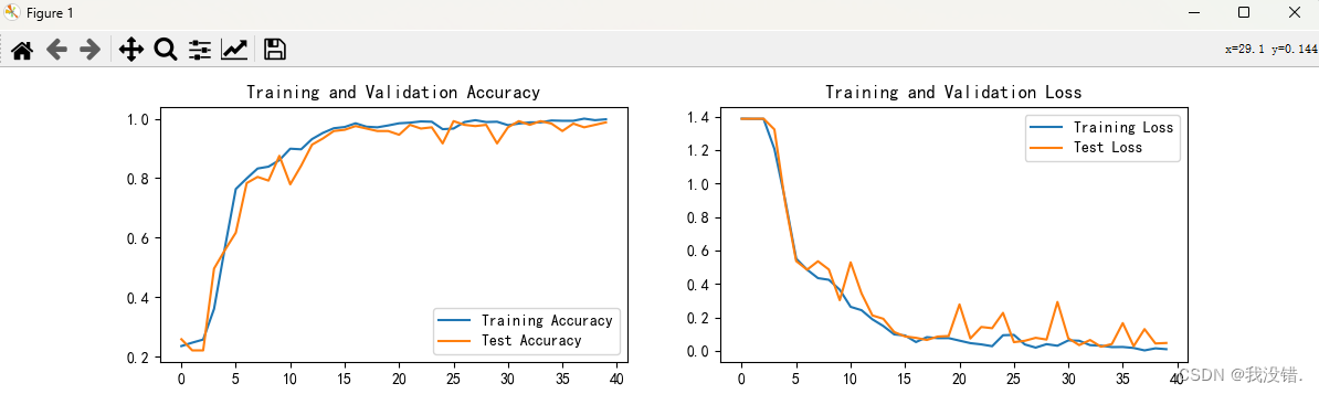


 4842
4842

 被折叠的 条评论
为什么被折叠?
被折叠的 条评论
为什么被折叠?
 到【灌水乐园】发言


