


文章目录
一、深度卷积神经网络AlexNet
1.理论知识
ImageNet(2010)
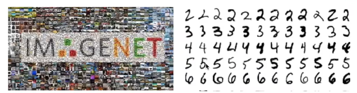
| 图片 | 自然物体的彩色图片 | 手写数字的黑色图片 |
|---|---|---|
| 大小 | 468 * 387 | 28*28 |
| 样本数 | 1.2M | 60K |
| 类数 | 1000 | 10 |
AlexNet
- AlexNet赢了2012ImageNet竞赛
- 更深更大的LeNet
- 主要改进:
- 丢弃法
- ReLu
- MaxPooling
- 计算机视觉方法论的改变

AlexNet架构
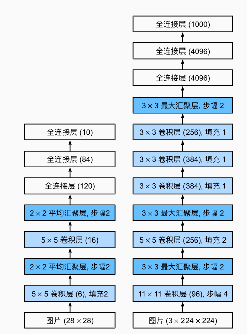
左边是LeNet.右边是AlexNet架构 - 激活函数从Sigmoid变到了ReLu(减缓梯度消失)
- 隐藏全连接层后加入了丢弃层
- 数据增强
2.代码
AlexNet原文使用的是ImageNet图像,但是为了方便我们使用Fashion-MNIST数据集。

1.定义网络
原本ImageNet为彩色图片,所以有三个通道,但是我们此时使用的数据集是灰度图,所以第一个卷积层的输入通道数为1。
    import torch
    from torch import nn
    from d2l import torch as d2l

    net = nn.Sequential(
        # 这里使用一个11*11的更大窗口来捕捉对象。
        # 同时,步幅为4,以减少输出的高度和宽度。
        # 另外,输出通道的数目远大于LeNet
        nn.Conv2d(1, 96, kernel_size=11, stride=4, padding=1), nn.ReLU(),
        nn.MaxPool2d(kernel_size=3, stride=2),
        # 减小卷积窗口,使用填充为2来使得输入与输出的高和宽一致,且增大输出通道数
        nn.Conv2d(96, 256, kernel_size=5, padding=2), nn.ReLU(),
        nn.MaxPool2d(kernel_size=3, stride=2),
        # 使用三个连续的卷积层和较小的卷积窗口。
        # 除了最后的卷积层,输出通道的数量进一步增加。
        # 在前两个卷积层之后,汇聚层不用于减少输入的高度和宽度
        nn.Conv2d(256, 384, kernel_size=3, padding=1), nn.ReLU(),
        nn.Conv2d(384, 384, kernel_size=3, padding=1), nn.ReLU(),
        nn.Conv2d(384, 256, kernel_size=3, padding=1),nn.ReLU(),
        nn.MaxPool2d(kernel_size=3, stride=2),
        nn.Flatten(),
        # 这里,全连接层的输出数量是LeNet中的好几倍。使用dropout层来减轻过拟合
        nn.Linear(6400, 4096), nn.ReLU(),
        nn.Dropout(p=0.5),
        nn.Linear(4096, 4096), nn.ReLU(),
        nn.Dropout(p=0.5),
        # 最后是输出层。由于这里使用Fashion-MNIST,所以用类别数为10,而非论文中的1000
        nn.Linear(4096, 10))
2.构造一个高和宽都为224的单通道数据,观察网络结构输出
X = torch.randn(1, 1, 224, 224)
for layer in net:
    X=layer(X)
    print(layer.__class__.__name__,'output shape:\t',X.shape)
Conv2d output shape:	 torch.Size([1, 96, 54, 54])
ReLU output shape:	 torch.Size([1, 96, 54, 54])
MaxPool2d output shape:	 torch.Size([1, 96, 26, 26])
Conv2d output shape:	 torch.Size([1, 256, 26, 26])
ReLU output shape:	 torch.Size([1, 256, 26, 26])
MaxPool2d output shape:	 torch.Size([1, 256, 12, 12])
Conv2d output shape:	 torch.Size([1, 384, 12, 12])
ReLU output shape:	 torch.Size([1, 384, 12, 12])
Conv2d output shape:	 torch.Size([1, 384, 12, 12])
ReLU output shape:	 torch.Size([1, 384, 12, 12])
Conv2d output shape:	 torch.Size([1, 256, 12, 12])
ReLU output shape:	 torch.Size([1, 256, 12, 12])
MaxPool2d output shape:	 torch.Size([1, 256, 5, 5])
Flatten output shape:	 torch.Size([1, 6400])
Linear output shape:	 torch.Size([1, 4096])
ReLU output shape:	 torch.Size([1, 4096])
Dropout output shape:	 torch.Size([1, 4096])
Linear output shape:	 torch.Size([1, 4096])
ReLU output shape:	 torch.Size([1, 4096])
Dropout output shape:	 torch.Size([1, 4096])
Linear output shape:	 torch.Size([1, 10])
3.读取数据集
Fashion-MNIST图像的分辨率(像素)低于ImageNet图像,需要增加到224*224
batch_size = 1
train_iter, test_iter = d2l.load_data_fashion_mnist(batch_size, resize=224)
train_iter.num_workers = 0
test_iter.num_workers = 0
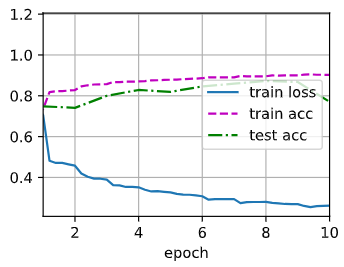
4.训练
lr, num_epochs = 0.01, 10
d2l.train_ch6(net, train_iter, test_iter, num_epochs, lr, d2l.try_gpu())
二、使用块的网络VGG
1.定义函数实现VGG块
import torch
from torch import nn
from d2l import torch as d2l

def vgg_block(num_convs, in_channels, out_channels):
    layers = []
    for _ in range(num_convs):
        layers.append(nn.Conv2d(in_channels, out_channels,
                               kernel_size=3, padding=1))
        layers.append(nn.ReLU())
        in_channels = out_channels
    layers.append(nn.MaxPool2d(kernel_size=2, stride=2))
    return nn.Sequential(*layers)
2.VGG网络

VGG网络可以分别两部分:卷积层和汇聚层+全连接层
# VGG网络
# 超参数conv_arch制定了VGG块里卷积层个数和输出通道数
conv_arch = ((1,64), (1, 128), (2, 256), (2, 512), (2, 512))
# VGG-11:8个卷积层+3个全连接层
def vgg(conv_arch):
    conv_blks = []
    in_channels = 1
    # 卷积层部分
    for (num_convs, out_channels) in conv_arch:
        conv_blks.append(vgg_block(num_convs, in_channels, out_channels))
        in_channels = out_channels

    return nn.Sequential(
        *conv_blks, nn.Flatten(),
        # 全连接层部分
        nn.Linear(out_channels * 7 * 7, 4096), nn.ReLU(), nn.Dropout(0.5),
        nn.Linear(4096, 4096), nn.ReLU(), nn.Dropout(0.5),
        nn.Linear(4096, 10))

net = vgg(conv_arch)
3.观察网络结构
X = torch.randn(size=(1, 1, 224, 224))
for blk in net:
    X = blk(X)
    print(blk.__class__.__name__,'output shape:\t',X.shape)
Sequential output shape:	 torch.Size([1, 64, 112, 112])
Sequential output shape:	 torch.Size([1, 128, 56, 56])
Sequential output shape:	 torch.Size([1, 256, 28, 28])
Sequential output shape:	 torch.Size([1, 512, 14, 14])
Sequential output shape:	 torch.Size([1, 512, 7, 7])
Flatten output shape:	 torch.Size([1, 25088])
Linear output shape:	 torch.Size([1, 4096])
ReLU output shape:	 torch.Size([1, 4096])
Dropout output shape:	 torch.Size([1, 4096])
Linear output shape:	 torch.Size([1, 4096])
ReLU output shape:	 torch.Size([1, 4096])
Dropout output shape:	 torch.Size([1, 4096])
Linear output shape:	 torch.Size([1, 10])
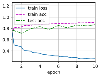
4.训练模型
# 训练模型

ratio = 4
small_conv_arch = [(pair[0], pair[1] // ratio) for pair in conv_arch]
net = vgg(small_conv_arch)
lr, num_epochs, batch_size = 0.05, 10, 128
train_iter, test_iter = d2l.load_data_fashion_mnist(batch_size, resize=224)
test_iter.num_workers = 0
test_iter.num_workers = 0
d2l.train_ch6(net, train_iter, test_iter, num_epochs, lr, d2l.try_gpu())
(;´༎ຶД༎ຶ`)
三、网络中的网络(NiN)
1.理论
全连接层的问题

NiN块
- 一个卷积层后跟两个全连接层
- 步幅1,无填充,输出形状跟卷积层输出一样
- 起到全连接层的作用

NiN架构
- 无全连接层
- 交替使用NiN块和步幅为2的最大池化层
- 逐步减小高宽和增大通道数
- 最后使用全局平均池化层得到输出
- 其输出通道数是类别数

- 其输出通道数是类别数
[总结]
- NiN块使用卷积层加两个1x1卷积层
- 后者对每个像素增加了非线性性
- NiN使用全局平均池化层来代替VGG和AlexNet中的全连接层
- 不容易过拟合,更少的参数个数
2.代码
import torch
from torch import nn
from d2l import torch as d2l

def nin_block(in_channels, out_channels, kernel_size, strides, padding):
    return nn.Sequential(
        nn.Conv2d(in_channels, out_channels, kernel_size, strides, padding),
        nn.ReLU(), nn.Conv2d(out_channels, out_channels, kernel_size=1),
        nn.ReLU(), nn.Conv2d(out_channels, out_channels, kernel_size=1),
        nn.ReLU())
# NiN模型
net = nn.Sequential(
    nin_block(1, 96, kernel_size=11, strides=4, padding=0),
    nn.MaxPool2d(3, stride=2),
    nin_block(96, 256, kernel_size=5, strides=1, padding=2),
    nn.MaxPool2d(3, stride=2),
    nin_block(256, 384, kernel_size=3, strides=1, padding=1),
    nn.MaxPool2d(3, stride=2), nn.Dropout(0.5),
    nin_block(384, 10, kernel_size=3, strides=1, padding=1),
    nn.AdaptiveAvgPool2d((1, 1)),
    nn.Flatten())
# 查看网络结构
X = torch.randn(size=(1, 1, 224, 224))
for layer in net:
    X = layer(X)
    print(layer.__class__.__name__,'output shape:\t', X.shape)
Sequential output shape:	 torch.Size([1, 96, 54, 54])
MaxPool2d output shape:	 torch.Size([1, 96, 26, 26])
Sequential output shape:	 torch.Size([1, 256, 26, 26])
MaxPool2d output shape:	 torch.Size([1, 256, 12, 12])
Sequential output shape:	 torch.Size([1, 384, 12, 12])
MaxPool2d output shape:	 torch.Size([1, 384, 5, 5])
Dropout output shape:	 torch.Size([1, 384, 5, 5])
Sequential output shape:	 torch.Size([1, 10, 5, 5])
AdaptiveAvgPool2d output shape:	 torch.Size([1, 10, 1, 1])
Flatten output shape:	 torch.Size([1, 10])
# 训练模型
lr, num_epochs, batch_size = 0.1, 10, 128
train_iter, test_iter = d2l.load_data_fashion_mnist(batch_size, resize=224)
train_iter.num_workers = 0
test_iter.num_workers = 0
d2l.train_ch6(net, train_iter, test_iter, num_epochs, lr, torch.device('cpu'))
四、含并行结的网络(GoogLeNet)
GoogLeNet基本的卷积块被称为Inception块。如下图由四条并行路径组成,最后将每条路线的输出在通道维度上连结,构成Inception块的输出。高宽不变,变得是通道数。

- 可以通过降低通道数来控制模型复杂度
- 每条路上通道数可能不同
GoogLeNet模型

- Inception块用4条不同超参数的卷积层和池化层的路来抽取不同的信息
- 它的一个主要优点是模型参数小,计算复杂度低
- GoogleNet使用了9个Inception块,是第一个达到上百层的网络
- 后续有一系列改进
2.代码
1.实现Inception块
import torch
from torch import nn
from torch.nn import functional as F
from d2l import torch as d2l


class Inception(nn.Module):
    # c1--c4是每条路径的输出通道数
    def __init__(self, in_channels, c1, c2, c3, c4, **kwargs):
        super(Inception, self).__init__(**kwargs)
        # 线路1,单1x1卷积层
        self.p1_1 = nn.Conv2d(in_channels, c1, kernel_size=1)
        # 线路2,1x1卷积层后接3x3卷积层
        self.p2_1 = nn.Conv2d(in_channels, c2[0], kernel_size=1)
        self.p2_2 = nn.Conv2d(c2[0], c2[1], kernel_size=3, padding=1)
        # 线路3,1x1卷积层后接5x5卷积层
        self.p3_1 = nn.Conv2d(in_channels, c3[0], kernel_size=1)
        self.p3_2 = nn.Conv2d(c3[0], c3[1], kernel_size=5, padding=2)
        # 线路4,3x3最大汇聚层后接1x1卷积层
        self.p4_1 = nn.MaxPool2d(kernel_size=3, stride=1, padding=1)
        self.p4_2 = nn.Conv2d(in_channels, c4, kernel_size=1)

    def forward(self, x):
        p1 = F.relu(self.p1_1(x))
        p2 = F.relu(self.p2_2(F.relu(self.p2_1(x))))
        p3 = F.relu(self.p3_2(F.relu(self.p3_1(x))))
        p4 = F.relu(self.p4_2(self.p4_1(x)))
        # 在通道维度上连结输出
        return torch.cat((p1, p2, p3, p4), dim=1)
b1 = nn.Sequential(nn.Conv2d(1, 64, kernel_size=7, stride=2, padding=3),
                   nn.ReLU(),
                   nn.MaxPool2d(kernel_size=3, stride=2, padding=1))
# 第二个模块使用两个卷积层:
# 第一个卷积层是64个通道、卷积层;
# 第二个卷积层使用将通道数量增加三倍的卷积层。

b2 = nn.Sequential(nn.Conv2d(64, 64, kernel_size=1),
                  nn.ReLU(),
                  nn.Conv2d(64, 192, kernel_size=3, padding=1),
                  nn.ReLU(),
                  nn.MaxPool2d(kernel_size=3, stride=2, padding=1))
# 第五模块包含输出通道数为256+320+128+128=832和384+384+128+128=1024的
# 两个Inception
b5 = nn.Sequential(Inception(832, 256, (160, 320), (32, 128), 128),
                   Inception(832, 384, (192, 384), (48, 128), 128),
                   nn.AdaptiveAvgPool2d((1, 1)),
                   nn.Flatten())

net = nn.Sequential(b1, b2, b3, b4, b5, nn.Linear(1024, 10))
# 第三个模块串联两个完整的Inception块
b3 = nn.Sequential(Inception(192, 64, (96, 128), (16, 32), 32),
                   Inception(256, 128, (128, 192), (32, 96), 64),
                   nn.MaxPool2d(kernel_size=3, stride=2, padding=1))
# 第四模块
b4 = nn.Sequential(Inception(480, 192, (96, 208), (16, 48), 64),
                   Inception(512, 160, (112, 224), (24, 64), 64),
                   Inception(512, 128, (128, 256), (24, 64), 64),
                   Inception(512, 112, (144, 288), (32, 64), 64),
                   Inception(528, 256, (160, 320), (32, 128), 128),
                   nn.MaxPool2d(kernel_size=3, stride=2, padding=1)
                  )
# 为了使Fashion-MNIST上的训练短小,将输入的高和宽从224降到96
X = torch.rand(size=(1, 1, 96, 96))
for layer in net:
    X = layer(X)
    print(layer.__class__.__name__,'output shape:\t', X.shape)
Sequential output shape:	 torch.Size([1, 64, 24, 24])
Sequential output shape:	 torch.Size([1, 192, 12, 12])
Sequential output shape:	 torch.Size([1, 480, 6, 6])
Sequential output shape:	 torch.Size([1, 832, 3, 3])
Sequential output shape:	 torch.Size([1, 1024])
Linear output shape:	 torch.Size([1, 10])
训练模型
# 训练
lr, num_epochs, batch_size = 0.1, 10, 128
train_iter, test_iter = d2l.load_data_fashion_mnist(batch_size, resize=96)
train_iter.num_workers = 0
test_iter.num_workers = 0
d2l.train_ch6(net, train_iter, test_iter, num_epochs, lr, torch.device('cpu'))
五、批量归一化
1.理论

- 损失出现在最后,后面的层训练较快
- 数据在底部
- 底部的层训练较慢
- 底部层一变化,所有都得跟着变
- 最后的那些层需要重新学习多次
- 导致收敛变慢
- 我们可以在学习底层的时候避免变化顶层吗?
批量归一化
- 固定小批量里面的均值和方差

然后再做额外的调整(可学习的参数)

批量归一化层

批量归一化在做什么? - 最初论文是想用它来减少内部协变量转移
- 后续有论文指出它可能就是通过在每个小批量里加入噪音来控制模型复杂度
- 因此没必要跟丢弃法混合使用
【总结】
- 批量归一化固定小批量中的均值和方差,然后学习出适合的偏移和缩放
- 可以加速收敛速度,但一般不改变模型精度
2.代码
import torch
from torch import nn
from d2l import torch as d2l


def batch_norm(X, gamma, beta, moving_mean, moving_var, eps, momentum):
    # 通过is_grad_enabled来判断当前模式是训练模式还是预测模式
    if not torch.is_grad_enabled():
        # 如果是在预测模式下,直接使用传入的移动平均所得的均值和方差
        X_hat = (X - moving_mean) / torch.sqrt(moving_var + eps)
    else:
        assert len(X.shape) in (2, 4)
        if len(X.shape) == 2:
            # 使用全连接层的情况,计算特征维上的均值和方差
            mean = X.mean(dim=0)
            var = ((X - mean) ** 2).mean(dim=0)
        else:
            # 使用二维卷积层的情况,计算通道维上(axis=1)的均值和方差。
            # 这里我们需要保持X的形状以便后面可以做广播运算
            mean = X.mean(dim=(0, 2, 3), keepdim=True)
            var = ((X - mean) ** 2).mean(dim=(0, 2, 3), keepdim=True)
        # 训练模式下,用当前的均值和方差做标准化
        X_hat = (X - mean) / torch.sqrt(var + eps)
        # 更新移动平均的均值和方差
        moving_mean = momentum * moving_mean + (1.0 - momentum) * mean
        moving_var = momentum * moving_var + (1.0 - momentum) * var
    Y = gamma * X_hat + beta  # 缩放和移位
    return Y, moving_mean.data, moving_var.data
#
class BatchNorm(nn.Module):
    # num_features: 完全连接层的输出数量或卷积层的输出通道数
    # num_dims: 2表示完全连接层, 4表示卷积层
    def __init__(self, num_features, num_dims):
        super().__init__()
        if num_dims == 2:
            shape = (1, num_features)
        else:
            shape = (1, num_features, 1, 1)
        # 参与求梯度和迭代的拉伸和偏移参数, 分别初始化成1和0
        self.gamma = nn.Parameter(torch.ones(shape))
        self.beta = nn.Parameter(torch.zeros(shape))
        # 非模型参数的变量初始化为0和1
        self.moving_mean = torch.zeros(shape)
        self.moving_var = torch.ones(shape)

    def forward(self, X):
        # 如果X不在内存上, 将moving_mean和moving_var复制到X所在显存上
        if self.moving_mean.device != X.device:
            self.moving_mean = self.moving_mean.to(X.device)
            self.moving_var = self.moving_var.to(X.device)
        # 保存更新过的moving_mean和moving_var
        Y, self.moving_mean, self.moving_var = batch_norm(
            X, self.gamma, self.beta, self.moving_mean,
            self.moving_var, eps=1e-5, momentum=0.9)
        return Y
# 使用批量规范化层的LeNet
# 批量规范化是在卷积层或全连接层之后、相应的激活函数之前
net = nn.Sequential(
    nn.Conv2d(1, 6, kernel_size=5), BatchNorm(6, num_dims=4), nn.Sigmoid(),
    nn.AvgPool2d(kernel_size=2, stride=2),
    nn.Conv2d(6, 16, kernel_size=5), BatchNorm(16, num_dims=4), nn.Sigmoid(),
    nn.AvgPool2d(kernel_size=2, stride=2), nn.Flatten(),
    nn.Linear(16*4*4, 120), BatchNorm(120, num_dims=2), nn.Sigmoid(),
    nn.Linear(120, 84), BatchNorm(84, num_dims=2), nn.Sigmoid(),
    nn.Linear(84,10))
# 训练,但是lr比之前大很多
lr, num_epochs, batch_size = 1, 10, 256
train_iter, test_iter = d2l.load_data_fashion_mnist(batch_size)
train_iter.num_workers = 0
test_iter.num_workers = 0
d2l.train_ch6(net, train_iter, test_iter, num_epochs, lr,  d2l.try_gpu())
loss 0.262, train acc 0.902, test acc 0.770
29170.7 examples/sec on cuda:0
# 第一个批量规范化层中学到的拉伸参数gamma和偏移参数beta
net[1].gamma.reshape((-1,)), net[1].beta.reshape((-1,))
(tensor([0.8503, 2.7909, 2.1335, 2.1349, 4.4349, 3.4243],
grad_fn=),
tensor([ 1.1721, 1.3393, 2.7016, 1.9772, -2.3293, 2.4437],
grad_fn=))
简明实现
net = nn.Sequential(
    nn.Conv2d(1, 6, kernel_size=5), nn.BatchNorm2d(6), nn.Sigmoid(),
    nn.AvgPool2d(kernel_size=2, stride=2),
    nn.Conv2d(6, 16, kernel_size=5), nn.BatchNorm2d(16), nn.Sigmoid(),
    nn.AvgPool2d(kernel_size=2, stride=2), nn.Flatten(),
    nn.Linear(256, 120), nn.BatchNorm1d(120), nn.Sigmoid(),
    nn.Linear(120, 84), nn.BatchNorm1d(84), nn.Sigmoid(),
    nn.Linear(84, 10))
d2l.train_ch6(net, train_iter, test_iter, num_epochs, lr, d2l.try_gpu())
loss 0.262, train acc 0.904, test acc 0.868
28742.0 examples/sec on cuda:0
六、残差网络ResNet
残差块

- 串联一个层改变函数类,我们希望能扩大函数类
- 残差块加入快速通道来得到f(x)=x+g(x)的结构
ResNet块细节

ResNet架构

- 残差块使得很深的网络更加容易训练
- 甚至可以训练一千层的网络
- 残差网络对随后的深层网络设计产生了深远影响,无论似乎卷积类网络还是全连接类网络。
【相关总结】
torch.nn.AdaptiveAvgPool2d()
torch.nn.AdaptiveAvgPool2d(output_size) :二维平均自适应池化,指定完输出的大小后,自动寻找适合的kernel_size和stride等参数。
import torch
import torch.nn as nn
m = nn.AdaptiveAvgPool2d((2,3))
input = torch.randn(1, 3, 4)
output = m(input)
print(output)
tensor([[[-0.8876, -0.7412, 0.0479],
[-0.3545, -0.6551, 0.0245]]])


 174
174


 被折叠的 条评论
为什么被折叠?
被折叠的 条评论
为什么被折叠?
 到【灌水乐园】发言


